Welcome to MMDetection3D’s documentation!
Prerequisites
Linux or macOS (Windows is in experimental support)
Python 3.6+
PyTorch 1.3+
CUDA 9.2+ (If you build PyTorch from source, CUDA 9.0 is also compatible)
GCC 5+
The required versions of MMCV, MMDetection and MMSegmentation for different versions of MMDetection3D are as below. Please install the correct version of MMCV, MMDetection and MMSegmentation to avoid installation issues.
| MMDetection3D version | MMDetection version | MMSegmentation version | MMCV version |
|---|---|---|---|
| master | mmdet>=2.19.0, <=3.0.0 | mmseg>=0.20.0, <=1.0.0 | mmcv-full>=1.4.8, <=1.5.0 |
| v1.0.0rc1 | mmdet>=2.19.0, <=3.0.0 | mmseg>=0.20.0, <=1.0.0 | mmcv-full>=1.4.8, <=1.5.0 |
| v1.0.0rc0 | mmdet>=2.19.0, <=3.0.0 | mmseg>=0.20.0, <=1.0.0 | mmcv-full>=1.3.17, <=1.5.0 |
| 0.18.1 | mmdet>=2.19.0, <=3.0.0 | mmseg>=0.20.0, <=1.0.0 | mmcv-full>=1.3.17, <=1.5.0 |
| 0.18.0 | mmdet>=2.19.0, <=3.0.0 | mmseg>=0.20.0, <=1.0.0 | mmcv-full>=1.3.17, <=1.5.0 |
| 0.17.3 | mmdet>=2.14.0, <=3.0.0 | mmseg>=0.14.1, <=1.0.0 | mmcv-full>=1.3.8, <=1.4.0 |
| 0.17.2 | mmdet>=2.14.0, <=3.0.0 | mmseg>=0.14.1, <=1.0.0 | mmcv-full>=1.3.8, <=1.4.0 |
| 0.17.1 | mmdet>=2.14.0, <=3.0.0 | mmseg>=0.14.1, <=1.0.0 | mmcv-full>=1.3.8, <=1.4.0 |
| 0.17.0 | mmdet>=2.14.0, <=3.0.0 | mmseg>=0.14.1, <=1.0.0 | mmcv-full>=1.3.8, <=1.4.0 |
| 0.16.0 | mmdet>=2.14.0, <=3.0.0 | mmseg>=0.14.1, <=1.0.0 | mmcv-full>=1.3.8, <=1.4.0 |
| 0.15.0 | mmdet>=2.14.0, <=3.0.0 | mmseg>=0.14.1, <=1.0.0 | mmcv-full>=1.3.8, <=1.4.0 |
| 0.14.0 | mmdet>=2.10.0, <=2.11.0 | mmseg==0.14.0 | mmcv-full>=1.3.1, <=1.4.0 |
| 0.13.0 | mmdet>=2.10.0, <=2.11.0 | Not required | mmcv-full>=1.2.4, <=1.4.0 |
| 0.12.0 | mmdet>=2.5.0, <=2.11.0 | Not required | mmcv-full>=1.2.4, <=1.4.0 |
| 0.11.0 | mmdet>=2.5.0, <=2.11.0 | Not required | mmcv-full>=1.2.4, <=1.3.0 |
| 0.10.0 | mmdet>=2.5.0, <=2.11.0 | Not required | mmcv-full>=1.2.4, <=1.3.0 |
| 0.9.0 | mmdet>=2.5.0, <=2.11.0 | Not required | mmcv-full>=1.2.4, <=1.3.0 |
| 0.8.0 | mmdet>=2.5.0, <=2.11.0 | Not required | mmcv-full>=1.1.5, <=1.3.0 |
| 0.7.0 | mmdet>=2.5.0, <=2.11.0 | Not required | mmcv-full>=1.1.5, <=1.3.0 |
| 0.6.0 | mmdet>=2.4.0, <=2.11.0 | Not required | mmcv-full>=1.1.3, <=1.2.0 |
| 0.5.0 | 2.3.0 | Not required | mmcv-full==1.0.5 |
Installation
Install MMDetection3D
Quick installation instructions script
Assuming that you already have CUDA 11.0 installed, here is a full script for quick installation of MMDetection3D with conda. Otherwise, you should refer to the step-by-step installation instructions in the next section.
conda create -n open-mmlab python=3.7 pytorch=1.9 cudatoolkit=11.0 torchvision -c pytorch -y
conda activate open-mmlab
pip3 install openmim
mim install mmcv-full
mim install mmdet
mim install mmsegmentation
git clone https://github.com/open-mmlab/mmdetection3d.git
cd mmdetection3d
pip3 install -e .
Step-by-step installation instructions
a. Create a conda virtual environment and activate it.
conda create -n open-mmlab python=3.7 -y
conda activate open-mmlab
b. Install PyTorch and torchvision following the official instructions.
conda install pytorch torchvision -c pytorch
Note: Make sure that your compilation CUDA version and runtime CUDA version match. You can check the supported CUDA version for precompiled packages on the PyTorch website.
E.g. 1 If you have CUDA 10.1 installed under /usr/local/cuda and would like to install
PyTorch 1.5, you need to install the prebuilt PyTorch with CUDA 10.1.
conda install pytorch==1.5.0 cudatoolkit=10.1 torchvision==0.6.0 -c pytorch
E.g. 2 If you have CUDA 9.2 installed under /usr/local/cuda and would like to install
PyTorch 1.3.1., you need to install the prebuilt PyTorch with CUDA 9.2.
conda install pytorch=1.3.1 cudatoolkit=9.2 torchvision=0.4.2 -c pytorch
If you build PyTorch from source instead of installing the prebuilt package, you can use more CUDA versions such as 9.0.
c. Install MMCV. mmcv-full is necessary since MMDetection3D relies on MMDetection, CUDA ops in mmcv-full are required.
e.g. The pre-build mmcv-full could be installed by running: (available versions could be found here)
pip install mmcv-full -f https://download.openmmlab.com/mmcv/dist/{cu_version}/{torch_version}/index.html
Please replace {cu_version} and {torch_version} in the url to your desired one. For example, to install the latest mmcv-full with CUDA 11 and PyTorch 1.7.0, use the following command:
pip install mmcv-full -f https://download.openmmlab.com/mmcv/dist/cu110/torch1.7.0/index.html
mmcv-full is only compiled on PyTorch 1.x.0 because the compatibility usually holds between 1.x.0 and 1.x.1. If your PyTorch version is 1.x.1, you can install mmcv-full compiled with PyTorch 1.x.0 and it usually works well.
# We can ignore the micro version of PyTorch
pip install mmcv-full -f https://download.openmmlab.com/mmcv/dist/cu110/torch1.7/index.html
See here for different versions of MMCV compatible to different PyTorch and CUDA versions. Optionally, you could also build the full version from source:
git clone https://github.com/open-mmlab/mmcv.git
cd mmcv
MMCV_WITH_OPS=1 pip install -e .  # package mmcv-full will be installed after this step
cd ..
Or directly run
pip install mmcv-full
d. Install MMDetection.
pip install mmdet
Optionally, you could also build MMDetection from source in case you want to modify the code:
git clone https://github.com/open-mmlab/mmdetection.git
cd mmdetection
git checkout v2.19.0  # switch to v2.19.0 branch
pip install -r requirements/build.txt
pip install -v -e .  # or "python setup.py develop"
e. Install MMSegmentation.
pip install mmsegmentation
Optionally, you could also build MMSegmentation from source in case you want to modify the code:
git clone https://github.com/open-mmlab/mmsegmentation.git
cd mmsegmentation
git checkout v0.20.0  # switch to v0.20.0 branch
pip install -e .  # or "python setup.py develop"
f. Clone the MMDetection3D repository.
git clone https://github.com/open-mmlab/mmdetection3d.git
cd mmdetection3d
g.Install build requirements and then install MMDetection3D.
pip install -v -e . # or "python setup.py develop"
Note:
The git commit id will be written to the version number with step d, e.g. 0.6.0+2e7045c. The version will also be saved in trained models. It is recommended that you run step d each time you pull some updates from github. If C++/CUDA codes are modified, then this step is compulsory.
Important: Be sure to remove the
./buildfolder if you reinstall mmdet with a different CUDA/PyTorch version.pip uninstall mmdet3d rm -rf ./build find . -name "*.so" | xargs rm
Following the above instructions, MMDetection3D is installed on
devmode, any local modifications made to the code will take effect without the need to reinstall it (unless you submit some commits and want to update the version number).If you would like to use
opencv-python-headlessinstead ofopencv-python, you can install it before installing MMCV.Some dependencies are optional. Simply running
pip install -v -e .will only install the minimum runtime requirements. To use optional dependencies likealbumentationsandimagecorruptionseither install them manually withpip install -r requirements/optional.txtor specify desired extras when callingpip(e.g.pip install -v -e .[optional]). Valid keys for the extras field are:all,tests,build, andoptional.The code can not be built for CPU only environment (where CUDA isn’t available) for now.
Another option: Docker Image
We provide a Dockerfile to build an image.
# build an image with PyTorch 1.6, CUDA 10.1
docker build -t mmdetection3d -f docker/Dockerfile .
Run it with
docker run --gpus all --shm-size=8g -it -v {DATA_DIR}:/mmdetection3d/data mmdetection3d
A from-scratch setup script
Here is a full script for setting up MMdetection3D with conda.
conda create -n open-mmlab python=3.7 -y
conda activate open-mmlab

# install latest PyTorch prebuilt with the default prebuilt CUDA version (usually the latest)
conda install -c pytorch pytorch torchvision -y

# install mmcv
pip install mmcv-full

# install mmdetection
pip install git+https://github.com/open-mmlab/mmdetection.git

# install mmsegmentation
pip install git+https://github.com/open-mmlab/mmsegmentation.git

# install mmdetection3d
git clone https://github.com/open-mmlab/mmdetection3d.git
cd mmdetection3d
pip install -v -e .
Using multiple MMDetection3D versions
The train and test scripts already modify the PYTHONPATH to ensure the script use the MMDetection3D in the current directory.
To use the default MMDetection3D installed in the environment rather than that you are working with, you can remove the following line in those scripts
PYTHONPATH="$(dirname $0)/..":$PYTHONPATH
Verification
Verify with point cloud demo
We provide several demo scripts to test a single sample. Pre-trained models can be downloaded from model zoo. To test a single-modality 3D detection on point cloud scenes:
python demo/pcd_demo.py ${PCD_FILE} ${CONFIG_FILE} ${CHECKPOINT_FILE} [--device ${GPU_ID}] [--score-thr ${SCORE_THR}] [--out-dir ${OUT_DIR}]
Examples:
python demo/pcd_demo.py demo/data/kitti/kitti_000008.bin configs/second/hv_second_secfpn_6x8_80e_kitti-3d-car.py checkpoints/hv_second_secfpn_6x8_80e_kitti-3d-car_20200620_230238-393f000c.pth
If you want to input a ply file, you can use the following function and convert it to bin format. Then you can use the converted bin file to generate demo.
Note that you need to install pandas and plyfile before using this script. This function can also be used for data preprocessing for training ply data.
import numpy as np
import pandas as pd
from plyfile import PlyData

def convert_ply(input_path, output_path):
    plydata = PlyData.read(input_path)  # read file
    data = plydata.elements[0].data  # read data
    data_pd = pd.DataFrame(data)  # convert to DataFrame
    data_np = np.zeros(data_pd.shape, dtype=np.float)  # initialize array to store data
    property_names = data[0].dtype.names  # read names of properties
    for i, name in enumerate(
            property_names):  # read data by property
        data_np[:, i] = data_pd[name]
    data_np.astype(np.float32).tofile(output_path)
Examples:
convert_ply('./test.ply', './test.bin')
If you have point clouds in other format (off, obj, etc.), you can use trimesh to convert them into ply.
import trimesh

def to_ply(input_path, output_path, original_type):
    mesh = trimesh.load(input_path, file_type=original_type)  # read file
    mesh.export(output_path, file_type='ply')  # convert to ply
Examples:
to_ply('./test.obj', './test.ply', 'obj')
More demos about single/multi-modality and indoor/outdoor 3D detection can be found in demo.
High-level APIs for testing point clouds
Synchronous interface
Here is an example of building the model and test given point clouds.
from mmdet3d.apis import init_model, inference_detector

config_file = 'configs/votenet/votenet_8x8_scannet-3d-18class.py'
checkpoint_file = 'checkpoints/votenet_8x8_scannet-3d-18class_20200620_230238-2cea9c3a.pth'

# build the model from a config file and a checkpoint file
model = init_model(config_file, checkpoint_file, device='cuda:0')

# test a single image and show the results
point_cloud = 'test.bin'
result, data = inference_detector(model, point_cloud)
# visualize the results and save the results in 'results' folder
model.show_results(data, result, out_dir='results')
Demo
Introduction
We provide scripts for multi-modality/single-modality (LiDAR-based/vision-based), indoor/outdoor 3D detection and 3D semantic segmentation demos. The pre-trained models can be downloaded from model zoo. We provide pre-processed sample data from KITTI, SUN RGB-D, nuScenes and ScanNet dataset. You can use any other data following our pre-processing steps.
Testing
3D Detection
Single-modality demo
To test a 3D detector on point cloud data, simply run:
python demo/pcd_demo.py ${PCD_FILE} ${CONFIG_FILE} ${CHECKPOINT_FILE} [--device ${GPU_ID}] [--score-thr ${SCORE_THR}] [--out-dir ${OUT_DIR}] [--show]
The visualization results including a point cloud and predicted 3D bounding boxes will be saved in ${OUT_DIR}/PCD_NAME, which you can open using MeshLab. Note that if you set the flag --show, the prediction result will be displayed online using Open3D.
Example on KITTI data using SECOND model:
python demo/pcd_demo.py demo/data/kitti/kitti_000008.bin configs/second/hv_second_secfpn_6x8_80e_kitti-3d-car.py checkpoints/hv_second_secfpn_6x8_80e_kitti-3d-car_20200620_230238-393f000c.pth
Example on SUN RGB-D data using VoteNet model:
python demo/pcd_demo.py demo/data/sunrgbd/sunrgbd_000017.bin configs/votenet/votenet_16x8_sunrgbd-3d-10class.py checkpoints/votenet_16x8_sunrgbd-3d-10class_20200620_230238-4483c0c0.pth
Remember to convert the VoteNet checkpoint if you are using mmdetection3d version >= 0.6.0. See its README for detailed instructions on how to convert the checkpoint.
Multi-modality demo
To test a 3D detector on multi-modality data (typically point cloud and image), simply run:
python demo/multi_modality_demo.py ${PCD_FILE} ${IMAGE_FILE} ${ANNOTATION_FILE} ${CONFIG_FILE} ${CHECKPOINT_FILE} [--device ${GPU_ID}] [--score-thr ${SCORE_THR}] [--out-dir ${OUT_DIR}] [--show]
where the ANNOTATION_FILE should provide the 3D to 2D projection matrix. The visualization results including a point cloud, an image, predicted 3D bounding boxes and their projection on the image will be saved in ${OUT_DIR}/PCD_NAME.
Example on KITTI data using MVX-Net model:
python demo/multi_modality_demo.py demo/data/kitti/kitti_000008.bin demo/data/kitti/kitti_000008.png demo/data/kitti/kitti_000008_infos.pkl configs/mvxnet/dv_mvx-fpn_second_secfpn_adamw_2x8_80e_kitti-3d-3class.py checkpoints/dv_mvx-fpn_second_secfpn_adamw_2x8_80e_kitti-3d-3class_20200621_003904-10140f2d.pth
Example on SUN RGB-D data using ImVoteNet model:
python demo/multi_modality_demo.py demo/data/sunrgbd/sunrgbd_000017.bin demo/data/sunrgbd/sunrgbd_000017.jpg demo/data/sunrgbd/sunrgbd_000017_infos.pkl configs/imvotenet/imvotenet_stage2_16x8_sunrgbd-3d-10class.py checkpoints/imvotenet_stage2_16x8_sunrgbd-3d-10class_20210323_184021-d44dcb66.pth
Monocular 3D Detection
To test a monocular 3D detector on image data, simply run:
python demo/mono_det_demo.py ${IMAGE_FILE} ${ANNOTATION_FILE} ${CONFIG_FILE} ${CHECKPOINT_FILE} [--device ${GPU_ID}] [--out-dir ${OUT_DIR}] [--show]
where the ANNOTATION_FILE should provide the 3D to 2D projection matrix (camera intrinsic matrix). The visualization results including an image and its predicted 3D bounding boxes projected on the image will be saved in ${OUT_DIR}/PCD_NAME.
Example on nuScenes data using FCOS3D model:
python demo/mono_det_demo.py demo/data/nuscenes/n015-2018-07-24-11-22-45+0800__CAM_BACK__1532402927637525.jpg demo/data/nuscenes/n015-2018-07-24-11-22-45+0800__CAM_BACK__1532402927637525_mono3d.coco.json configs/fcos3d/fcos3d_r101_caffe_fpn_gn-head_dcn_2x8_1x_nus-mono3d_finetune.py checkpoints/fcos3d_r101_caffe_fpn_gn-head_dcn_2x8_1x_nus-mono3d_finetune_20210717_095645-8d806dc2.pth
Note that when visualizing results of monocular 3D detection for flipped images, the camera intrinsic matrix should also be modified accordingly. See more details and examples in PR #744.
3D Segmentation
To test a 3D segmentor on point cloud data, simply run:
python demo/pc_seg_demo.py ${PCD_FILE} ${CONFIG_FILE} ${CHECKPOINT_FILE} [--device ${GPU_ID}] [--out-dir ${OUT_DIR}] [--show]
The visualization results including a point cloud and its predicted 3D segmentation mask will be saved in ${OUT_DIR}/PCD_NAME.
Example on ScanNet data using PointNet++ (SSG) model:
python demo/pc_seg_demo.py demo/data/scannet/scene0000_00.bin configs/pointnet2/pointnet2_ssg_16x2_cosine_200e_scannet_seg-3d-20class.py checkpoints/pointnet2_ssg_16x2_cosine_200e_scannet_seg-3d-20class_20210514_143644-ee73704a.pth
Model Zoo
Common settings
We use distributed training.
For fair comparison with other codebases, we report the GPU memory as the maximum value of
torch.cuda.max_memory_allocated()for all 8 GPUs. Note that this value is usually less than whatnvidia-smishows.We report the inference time as the total time of network forwarding and post-processing, excluding the data loading time. Results are obtained with the script benchmark.py which computes the average time on 2000 images.
Baselines
SECOND
Please refer to SECOND for details. We provide SECOND baselines on KITTI and Waymo datasets.
PointPillars
Please refer to PointPillars for details. We provide pointpillars baselines on KITTI, nuScenes, Lyft, and Waymo datasets.
VoteNet
Please refer to VoteNet for details. We provide VoteNet baselines on ScanNet and SUNRGBD datasets.
Dynamic Voxelization
Please refer to Dynamic Voxelization for details.
RegNetX
Please refer to RegNet for details. We provide pointpillars baselines with RegNetX backbones on nuScenes and Lyft datasets currently.
nuImages
We also support baseline models on nuImages dataset. Please refer to nuImages for details. We report Mask R-CNN, Cascade Mask R-CNN and HTC results currently.
CenterPoint
Please refer to CenterPoint for details.
SSN
Please refer to SSN for details. We provide pointpillars with shape-aware grouping heads used in SSN on the nuScenes and Lyft datasets currently.
ImVoteNet
Please refer to ImVoteNet for details. We provide ImVoteNet baselines on SUNRGBD dataset.
PointNet++
Please refer to PointNet++ for details. We provide PointNet++ baselines on ScanNet and S3DIS datasets.
Group-Free-3D
Please refer to Group-Free-3D for details. We provide Group-Free-3D baselines on ScanNet dataset.
ImVoxelNet
Please refer to ImVoxelNet for details. We provide ImVoxelNet baselines on KITTI dataset.
Mixed Precision (FP16) Training
Please refer to Mixed Precision (FP16) Training on PointPillars for details.
Dataset Preparation
Before Preparation
It is recommended to symlink the dataset root to $MMDETECTION3D/data.
If your folder structure is different from the following, you may need to change the corresponding paths in config files.
mmdetection3d
├── mmdet3d
├── tools
├── configs
├── data
│   ├── nuscenes
│   │   ├── maps
│   │   ├── samples
│   │   ├── sweeps
│   │   ├── v1.0-test
|   |   ├── v1.0-trainval
│   ├── kitti
│   │   ├── ImageSets
│   │   ├── testing
│   │   │   ├── calib
│   │   │   ├── image_2
│   │   │   ├── velodyne
│   │   ├── training
│   │   │   ├── calib
│   │   │   ├── image_2
│   │   │   ├── label_2
│   │   │   ├── velodyne
│   ├── waymo
│   │   ├── waymo_format
│   │   │   ├── training
│   │   │   ├── validation
│   │   │   ├── testing
│   │   │   ├── gt.bin
│   │   ├── kitti_format
│   │   │   ├── ImageSets
│   ├── lyft
│   │   ├── v1.01-train
│   │   │   ├── v1.01-train (train_data)
│   │   │   ├── lidar (train_lidar)
│   │   │   ├── images (train_images)
│   │   │   ├── maps (train_maps)
│   │   ├── v1.01-test
│   │   │   ├── v1.01-test (test_data)
│   │   │   ├── lidar (test_lidar)
│   │   │   ├── images (test_images)
│   │   │   ├── maps (test_maps)
│   │   ├── train.txt
│   │   ├── val.txt
│   │   ├── test.txt
│   │   ├── sample_submission.csv
│   ├── s3dis
│   │   ├── meta_data
│   │   ├── Stanford3dDataset_v1.2_Aligned_Version
│   │   ├── collect_indoor3d_data.py
│   │   ├── indoor3d_util.py
│   │   ├── README.md
│   ├── scannet
│   │   ├── meta_data
│   │   ├── scans
│   │   ├── scans_test
│   │   ├── batch_load_scannet_data.py
│   │   ├── load_scannet_data.py
│   │   ├── scannet_utils.py
│   │   ├── README.md
│   ├── sunrgbd
│   │   ├── OFFICIAL_SUNRGBD
│   │   ├── matlab
│   │   ├── sunrgbd_data.py
│   │   ├── sunrgbd_utils.py
│   │   ├── README.md
Download and Data Preparation
KITTI
Download KITTI 3D detection data HERE. Prepare KITTI data splits by running
mkdir ./data/kitti/ && mkdir ./data/kitti/ImageSets

# Download data split
wget -c  https://raw.githubusercontent.com/traveller59/second.pytorch/master/second/data/ImageSets/test.txt --no-check-certificate --content-disposition -O ./data/kitti/ImageSets/test.txt
wget -c  https://raw.githubusercontent.com/traveller59/second.pytorch/master/second/data/ImageSets/train.txt --no-check-certificate --content-disposition -O ./data/kitti/ImageSets/train.txt
wget -c  https://raw.githubusercontent.com/traveller59/second.pytorch/master/second/data/ImageSets/val.txt --no-check-certificate --content-disposition -O ./data/kitti/ImageSets/val.txt
wget -c  https://raw.githubusercontent.com/traveller59/second.pytorch/master/second/data/ImageSets/trainval.txt --no-check-certificate --content-disposition -O ./data/kitti/ImageSets/trainval.txt
Then generate info files by running
python tools/create_data.py kitti --root-path ./data/kitti --out-dir ./data/kitti --extra-tag kitti
In an environment using slurm, users may run the following command instead
sh tools/create_data.sh <partition> kitti
Waymo
Download Waymo open dataset V1.2 HERE and its data split HERE. Then put tfrecord files into corresponding folders in data/waymo/waymo_format/ and put the data split txt files into data/waymo/kitti_format/ImageSets. Download ground truth bin file for validation set HERE and put it into data/waymo/waymo_format/. A tip is that you can use gsutil to download the large-scale dataset with commands. You can take this tool as an example for more details. Subsequently, prepare waymo data by running
python tools/create_data.py waymo --root-path ./data/waymo/ --out-dir ./data/waymo/ --workers 128 --extra-tag waymo
Note that if your local disk does not have enough space for saving converted data, you can change the out-dir to anywhere else. Just remember to create folders and prepare data there in advance and link them back to data/waymo/kitti_format after the data conversion.
NuScenes
Download nuScenes V1.0 full dataset data HERE. Prepare nuscenes data by running
python tools/create_data.py nuscenes --root-path ./data/nuscenes --out-dir ./data/nuscenes --extra-tag nuscenes
Lyft
Download Lyft 3D detection data HERE. Prepare Lyft data by running
python tools/create_data.py lyft --root-path ./data/lyft --out-dir ./data/lyft --extra-tag lyft --version v1.01
python tools/data_converter/lyft_data_fixer.py --version v1.01 --root-folder ./data/lyft
Note that we follow the original folder names for clear organization. Please rename the raw folders as shown above. Also note that the second command serves the purpose of fixing a corrupted lidar data file. Please refer to the discussion here for more details.
S3DIS, ScanNet and SUN RGB-D
To prepare S3DIS data, please see its README.
To prepare ScanNet data, please see its README.
To prepare SUN RGB-D data, please see its README.
Customized Datasets
For using custom datasets, please refer to Tutorials 2: Customize Datasets.
1: Inference and train with existing models and standard datasets
Inference with existing models
Here we provide testing scripts to evaluate a whole dataset (SUNRGBD, ScanNet, KITTI, etc.).
For high-level apis easier to integrated into other projects and basic demos, please refer to Verification/Demo under Get Started.
Test existing models on standard datasets
single GPU
CPU
single node multiple GPU
multiple node
You can use the following commands to test a dataset.
# single-gpu testing
python tools/test.py ${CONFIG_FILE} ${CHECKPOINT_FILE} [--out ${RESULT_FILE}] [--eval ${EVAL_METRICS}] [--show] [--show-dir ${SHOW_DIR}]

# CPU: disable GPUs and run single-gpu testing script (experimental)
export CUDA_VISIBLE_DEVICES=-1
python tools/test.py ${CONFIG_FILE} ${CHECKPOINT_FILE} [--out ${RESULT_FILE}] [--eval ${EVAL_METRICS}] [--show] [--show-dir ${SHOW_DIR}]

# multi-gpu testing
./tools/dist_test.sh ${CONFIG_FILE} ${CHECKPOINT_FILE} ${GPU_NUM} [--out ${RESULT_FILE}] [--eval ${EVAL_METRICS}]
Note:
For now, CPU testing is only supported for SMOKE.
Optional arguments:
RESULT_FILE: Filename of the output results in pickle format. If not specified, the results will not be saved to a file.EVAL_METRICS: Items to be evaluated on the results. Allowed values depend on the dataset. Typically we default to use official metrics for evaluation on different datasets, so it can be simply set tomAPas a placeholder for detection tasks, which applies to nuScenes, Lyft, ScanNet and SUNRGBD. For KITTI, if we only want to evaluate the 2D detection performance, we can simply set the metric toimg_bbox(unstable, stay tuned). For Waymo, we provide both KITTI-style evaluation (unstable) and Waymo-style official protocol, corresponding to metrickittiandwaymorespectively. We recommend to use the default official metric for stable performance and fair comparison with other methods. Similarly, the metric can be set tomIoUfor segmentation tasks, which applies to S3DIS and ScanNet.--show: If specified, detection results will be plotted in the silient mode. It is only applicable to single GPU testing and used for debugging and visualization. This should be used with--show-dir.--show-dir: If specified, detection results will be plotted on the***_points.objand***_pred.objfiles in the specified directory. It is only applicable to single GPU testing and used for debugging and visualization. You do NOT need a GUI available in your environment for using this option.
Examples:
Assume that you have already downloaded the checkpoints to the directory checkpoints/.
Test VoteNet on ScanNet and save the points and prediction visualization results.
python tools/test.py configs/votenet/votenet_8x8_scannet-3d-18class.py \
    checkpoints/votenet_8x8_scannet-3d-18class_20200620_230238-2cea9c3a.pth \
    --show --show-dir ./data/scannet/show_results
Test VoteNet on ScanNet, save the points, prediction, groundtruth visualization results, and evaluate the mAP.
python tools/test.py configs/votenet/votenet_8x8_scannet-3d-18class.py \
    checkpoints/votenet_8x8_scannet-3d-18class_20200620_230238-2cea9c3a.pth \
    --eval mAP
    --eval-options 'show=True' 'out_dir=./data/scannet/show_results'
Test VoteNet on ScanNet (without saving the test results) and evaluate the mAP.
python tools/test.py configs/votenet/votenet_8x8_scannet-3d-18class.py \
    checkpoints/votenet_8x8_scannet-3d-18class_20200620_230238-2cea9c3a.pth \
    --eval mAP
Test SECOND on KITTI with 8 GPUs, and evaluate the mAP.
./tools/slurm_test.sh ${PARTITION} ${JOB_NAME} configs/second/hv_second_secfpn_6x8_80e_kitti-3d-3class.py \
    checkpoints/hv_second_secfpn_6x8_80e_kitti-3d-3class_20200620_230238-9208083a.pth \
    --out results.pkl --eval mAP
Test PointPillars on nuScenes with 8 GPUs, and generate the json file to be submit to the official evaluation server.
./tools/slurm_test.sh ${PARTITION} ${JOB_NAME} configs/pointpillars/hv_pointpillars_fpn_sbn-all_4x8_2x_nus-3d.py \
    checkpoints/hv_pointpillars_fpn_sbn-all_4x8_2x_nus-3d_20200620_230405-2fa62f3d.pth \
    --format-only --eval-options 'jsonfile_prefix=./pointpillars_nuscenes_results'
The generated results be under
./pointpillars_nuscenes_resultsdirectory.Test SECOND on KITTI with 8 GPUs, and generate the pkl files and submission data to be submit to the official evaluation server.
./tools/slurm_test.sh ${PARTITION} ${JOB_NAME} configs/second/hv_second_secfpn_6x8_80e_kitti-3d-3class.py \
    checkpoints/hv_second_secfpn_6x8_80e_kitti-3d-3class_20200620_230238-9208083a.pth \
    --format-only --eval-options 'pklfile_prefix=./second_kitti_results' 'submission_prefix=./second_kitti_results'
The generated results be under
./second_kitti_resultsdirectory.Test PointPillars on Lyft with 8 GPUs, generate the pkl files and make a submission to the leaderboard.
./tools/slurm_test.sh ${PARTITION} ${JOB_NAME} configs/pointpillars/hv_pointpillars_fpn_sbn-2x8_2x_lyft-3d.py \
    checkpoints/hv_pointpillars_fpn_sbn-2x8_2x_lyft-3d_latest.pth --out results/pp_lyft/results_challenge.pkl \
    --format-only --eval-options 'jsonfile_prefix=results/pp_lyft/results_challenge' \
    'csv_savepath=results/pp_lyft/results_challenge.csv'
Notice: To generate submissions on Lyft,
csv_savepathmust be given in the--eval-options. After generating the csv file, you can make a submission with kaggle commands given on the website.Note that in the config of Lyft dataset, the value of
ann_filekeyword intestisdata_root + 'lyft_infos_test.pkl', which is the official test set of Lyft without annotation. To test on the validation set, please change this todata_root + 'lyft_infos_val.pkl'.Test PointPillars on waymo with 8 GPUs, and evaluate the mAP with waymo metrics.
./tools/slurm_test.sh ${PARTITION} ${JOB_NAME} configs/pointpillars/hv_pointpillars_secfpn_sbn-2x16_2x_waymo-3d-car.py \
    checkpoints/hv_pointpillars_secfpn_sbn-2x16_2x_waymo-3d-car_latest.pth --out results/waymo-car/results_eval.pkl \
    --eval waymo --eval-options 'pklfile_prefix=results/waymo-car/kitti_results' \
    'submission_prefix=results/waymo-car/kitti_results'
Notice: For evaluation on waymo, please follow the instruction to build the binary file
compute_detection_metrics_mainfor metrics computation and put it intommdet3d/core/evaluation/waymo_utils/.(Sometimes when using bazel to buildcompute_detection_metrics_main, an error'round' is not a member of 'std'may appear. We just need to remove thestd::beforeroundin that file.)pklfile_prefixshould be given in the--eval-optionsfor the bin file generation. For metrics,waymois the recommended official evaluation prototype. Currently, evaluating with choicekittiis adapted from KITTI and the results for each difficulty are not exactly the same as the definition of KITTI. Instead, most of objects are marked with difficulty 0 currently, which will be fixed in the future. The reasons of its instability include the large computation for evaluation, the lack of occlusion and truncation in the converted data, different definition of difficulty and different methods of computing average precision.Test PointPillars on waymo with 8 GPUs, generate the bin files and make a submission to the leaderboard.
./tools/slurm_test.sh ${PARTITION} ${JOB_NAME} configs/pointpillars/hv_pointpillars_secfpn_sbn-2x16_2x_waymo-3d-car.py \
    checkpoints/hv_pointpillars_secfpn_sbn-2x16_2x_waymo-3d-car_latest.pth --out results/waymo-car/results_eval.pkl \
    --format-only --eval-options 'pklfile_prefix=results/waymo-car/kitti_results' \
    'submission_prefix=results/waymo-car/kitti_results'
Notice: After generating the bin file, you can simply build the binary file
create_submissionand use them to create a submission file by following the instruction. For evaluation on the validation set with the eval server, you can also use the same way to generate a submission.
Train predefined models on standard datasets
MMDetection3D implements distributed training and non-distributed training,
which uses MMDistributedDataParallel and MMDataParallel respectively.
All outputs (log files and checkpoints) will be saved to the working directory,
which is specified by work_dir in the config file.
By default we evaluate the model on the validation set after each epoch, you can change the evaluation interval by adding the interval argument in the training config.
evaluation = dict(interval=12) # This evaluate the model per 12 epoch.
Important: The default learning rate in config files is for 8 GPUs and the exact batch size is marked by the config’s file name, e.g. ‘2x8’ means 2 samples per GPU using 8 GPUs. According to the Linear Scaling Rule, you need to set the learning rate proportional to the batch size if you use different GPUs or images per GPU, e.g., lr=0.01 for 4 GPUs * 2 img/gpu and lr=0.08 for 16 GPUs * 4 img/gpu. However, since most of the models in this repo use ADAM rather than SGD for optimization, the rule may not hold and users need to tune the learning rate by themselves.
Train with a single GPU
python tools/train.py ${CONFIG_FILE} [optional arguments]
If you want to specify the working directory in the command, you can add an argument --work-dir ${YOUR_WORK_DIR}.
Training with CPU (experimental)
The process of training on the CPU is consistent with single GPU training. We just need to disable GPUs before the training process.
export CUDA_VISIBLE_DEVICES=-1
And then run the script of train with a single GPU.
Note:
For now, most of the point cloud related algorithms rely on 3D CUDA op, which can not be trained on CPU. Some monocular 3D object detection algorithms, like FCOS3D and SMOKE can be trained on CPU. We do not recommend users to use CPU for training because it is too slow. We support this feature to allow users to debug certain models on machines without GPU for convenience.
Train with multiple GPUs
./tools/dist_train.sh ${CONFIG_FILE} ${GPU_NUM} [optional arguments]
Optional arguments are:
--no-validate(not suggested): By default, the codebase will perform evaluation at every k (default value is 1, which can be modified like this) epochs during the training. To disable this behavior, use--no-validate.--work-dir ${WORK_DIR}: Override the working directory specified in the config file.--resume-from ${CHECKPOINT_FILE}: Resume from a previous checkpoint file.--options 'Key=value': Override some settings in the used config.
Difference between resume-from and load-from:
resume-fromloads both the model weights and optimizer status, and the epoch is also inherited from the specified checkpoint. It is usually used for resuming the training process that is interrupted accidentally.load-fromonly loads the model weights and the training epoch starts from 0. It is usually used for finetuning.
Train with multiple machines
If you run MMDetection3D on a cluster managed with slurm, you can use the script slurm_train.sh. (This script also supports single machine training.)
[GPUS=${GPUS}] ./tools/slurm_train.sh ${PARTITION} ${JOB_NAME} ${CONFIG_FILE} ${WORK_DIR}
Here is an example of using 16 GPUs to train Mask R-CNN on the dev partition.
GPUS=16 ./tools/slurm_train.sh dev pp_kitti_3class hv_pointpillars_secfpn_6x8_160e_kitti-3d-3class.py /nfs/xxxx/pp_kitti_3class
You can check slurm_train.sh for full arguments and environment variables.
If you launch with multiple machines simply connected with ethernet, you can simply run following commands:
On the first machine:
NNODES=2 NODE_RANK=0 PORT=$MASTER_PORT MASTER_ADDR=$MASTER_ADDR ./tools/dist_train.sh $CONFIG $GPUS
On the second machine:
NNODES=2 NODE_RANK=1 PORT=$MASTER_PORT MASTER_ADDR=$MASTER_ADDR ./tools/dist_train.sh $CONFIG $GPUS
Usually it is slow if you do not have high speed networking like InfiniBand.
Launch multiple jobs on a single machine
If you launch multiple jobs on a single machine, e.g., 2 jobs of 4-GPU training on a machine with 8 GPUs, you need to specify different ports (29500 by default) for each job to avoid communication conflict.
If you use dist_train.sh to launch training jobs, you can set the port in commands.
CUDA_VISIBLE_DEVICES=0,1,2,3 PORT=29500 ./tools/dist_train.sh ${CONFIG_FILE} 4
CUDA_VISIBLE_DEVICES=4,5,6,7 PORT=29501 ./tools/dist_train.sh ${CONFIG_FILE} 4
If you use launch training jobs with Slurm, there are two ways to specify the ports.
Set the port through
--options. This is more recommended since it does not change the original configs.CUDA_VISIBLE_DEVICES=0,1,2,3 GPUS=4 ./tools/slurm_train.sh ${PARTITION} ${JOB_NAME} config1.py ${WORK_DIR} --options 'dist_params.port=29500' CUDA_VISIBLE_DEVICES=4,5,6,7 GPUS=4 ./tools/slurm_train.sh ${PARTITION} ${JOB_NAME} config2.py ${WORK_DIR} --options 'dist_params.port=29501'
Modify the config files (usually the 6th line from the bottom in config files) to set different communication ports.
In
config1.py,dist_params = dict(backend='nccl', port=29500)
In
config2.py,dist_params = dict(backend='nccl', port=29501)
Then you can launch two jobs with
config1.pyandconfig2.py.CUDA_VISIBLE_DEVICES=0,1,2,3 GPUS=4 ./tools/slurm_train.sh ${PARTITION} ${JOB_NAME} config1.py ${WORK_DIR} CUDA_VISIBLE_DEVICES=4,5,6,7 GPUS=4 ./tools/slurm_train.sh ${PARTITION} ${JOB_NAME} config2.py ${WORK_DIR}
2: Train with customized datasets
In this note, you will know how to train and test predefined models with customized datasets. We use the Waymo dataset as an example to describe the whole process.
The basic steps are as below:
Prepare the customized dataset
Prepare a config
Train, test, inference models on the customized dataset.
Prepare the customized dataset
There are three ways to support a new dataset in MMDetection3D:
reorganize the dataset into existing format.
reorganize the dataset into a middle format.
implement a new dataset.
Usually we recommend to use the first two methods which are usually easier than the third.
In this note, we give an example for converting the data into KITTI format.
Note: We take Waymo as the example here considering its format is totally different from other existing formats. For other datasets using similar methods to organize data, like Lyft compared to nuScenes, it would be easier to directly implement the new data converter (for the second approach above) instead of converting it to another format (for the first approach above).
KITTI dataset format
Firstly, the raw data for 3D object detection from KITTI are typically organized as follows, where ImageSets contains split files indicating which files belong to training/validation/testing set, calib contains calibration information files, image_2 and velodyne include image data and point cloud data, and label_2 includes label files for 3D detection.
mmdetection3d
├── mmdet3d
├── tools
├── configs
├── data
│   ├── kitti
│   │   ├── ImageSets
│   │   ├── testing
│   │   │   ├── calib
│   │   │   ├── image_2
│   │   │   ├── velodyne
│   │   ├── training
│   │   │   ├── calib
│   │   │   ├── image_2
│   │   │   ├── label_2
│   │   │   ├── velodyne
Specific annotation format is described in the official object development kit. For example, it consists of the following labels:
#Values    Name      Description
----------------------------------------------------------------------------
   1    type         Describes the type of object: 'Car', 'Van', 'Truck',
                     'Pedestrian', 'Person_sitting', 'Cyclist', 'Tram',
                     'Misc' or 'DontCare'
   1    truncated    Float from 0 (non-truncated) to 1 (truncated), where
                     truncated refers to the object leaving image boundaries
   1    occluded     Integer (0,1,2,3) indicating occlusion state:
                     0 = fully visible, 1 = partly occluded
                     2 = largely occluded, 3 = unknown
   1    alpha        Observation angle of object, ranging [-pi..pi]
   4    bbox         2D bounding box of object in the image (0-based index):
                     contains left, top, right, bottom pixel coordinates
   3    dimensions   3D object dimensions: height, width, length (in meters)
   3    location     3D object location x,y,z in camera coordinates (in meters)
   1    rotation_y   Rotation ry around Y-axis in camera coordinates [-pi..pi]
   1    score        Only for results: Float, indicating confidence in
                     detection, needed for p/r curves, higher is better.
Assume we use the Waymo dataset. After downloading the data, we need to implement a function to convert both the input data and annotation format into the KITTI style. Then we can implement WaymoDataset inherited from KittiDataset to load the data and perform training and evaluation.
Specifically, we implement a waymo converter to convert Waymo data into KITTI format and a waymo dataset class to process it. Because we preprocess the raw data and reorganize it like KITTI, the dataset class could be implemented more easily by inheriting from KittiDataset. The last thing needed to be noted is the evaluation protocol you would like to use. Because Waymo has its own evaluation approach, we further incorporate it into our dataset class. Afterwards, users can successfully convert the data format and use WaymoDataset to train and evaluate the model.
For more details about the intermediate results of preprocessing of Waymo dataset, please refer to its tutorial.
Prepare a config
The second step is to prepare configs such that the dataset could be successfully loaded. In addition, adjusting hyperparameters is usually necessary to obtain decent performance in 3D detection.
Suppose we would like to train PointPillars on Waymo to achieve 3D detection for 3 classes, vehicle, cyclist and pedestrian, we need to prepare dataset config like this, model config like this and combine them like this, compared to KITTI dataset config, model config and overall.
Train a new model
To train a model with the new config, you can simply run
python tools/train.py configs/pointpillars/hv_pointpillars_secfpn_sbn_2x16_2x_waymoD5-3d-3class.py
For more detailed usages, please refer to the Case 1.
Test and inference
To test the trained model, you can simply run
python tools/test.py configs/pointpillars/hv_pointpillars_secfpn_sbn_2x16_2x_waymoD5-3d-3class.py work_dirs/hv_pointpillars_secfpn_sbn_2x16_2x_waymoD5-3d-3class/latest.pth --eval waymo
Note: To use Waymo evaluation protocol, you need to follow the tutorial and prepare files related to metrics computation as official instructions.
For more detailed usages for test and inference, please refer to the Case 1.
LiDAR-Based 3D Detection
LiDAR-based 3D detection is one of the most basic tasks supported in MMDetection3D. It expects the given model to take any number of points with features collected by LiDAR as input, and predict the 3D bounding boxes and category labels for each object of interest. Next, taking PointPillars on the KITTI dataset as an example, we will show how to prepare data, train and test a model on a standard 3D detection benchmark, and how to visualize and validate the results.
Data Preparation
To begin with, we need to download the raw data and reorganize the data in a standard way presented in the doc for data preparation. Note that for KITTI, we need extra txt files for data splits.
Due to different ways of organizing the raw data in different datasets, we typically need to collect the useful data information with a .pkl or .json file.
So after getting all the raw data ready, we need to run the scripts provided in the create_data.py for different datasets to generate data infos.
For example, for KITTI we need to run:
python tools/create_data.py kitti --root-path ./data/kitti --out-dir ./data/kitti --extra-tag kitti
Afterwards, the related folder structure should be as follows:
mmdetection3d
├── mmdet3d
├── tools
├── configs
├── data
│   ├── kitti
│   │   ├── ImageSets
│   │   ├── testing
│   │   │   ├── calib
│   │   │   ├── image_2
│   │   │   ├── velodyne
│   │   ├── training
│   │   │   ├── calib
│   │   │   ├── image_2
│   │   │   ├── label_2
│   │   │   ├── velodyne
│   │   ├── kitti_gt_database
│   │   ├── kitti_infos_train.pkl
│   │   ├── kitti_infos_trainval.pkl
│   │   ├── kitti_infos_val.pkl
│   │   ├── kitti_infos_test.pkl
│   │   ├── kitti_dbinfos_train.pkl
Training
Then let us train a model with provided configs for PointPillars. You can basically follow this tutorial for sample scripts when training with different GPU settings. Suppose we use 8 GPUs on a single machine with distributed training:
./tools/dist_train.sh configs/pointpillars/hv_pointpillars_secfpn_6x8_160e_kitti-3d-3class.py 8
Note that 6x8 in the config name refers to the training is completed with 8 GPUs and 6 samples on each GPU.
If your customized setting is different from this, sometimes you need to adjust the learning rate accordingly.
A basic rule can be referred to here.
Quantitative Evaluation
During training, the model checkpoints will be evaluated regularly according to the setting of evaluation = dict(interval=xxx) in the config.
We support official evaluation protocols for different datasets.
For KITTI, the model will be evaluated with mean average precision (mAP) with Intersection over Union (IoU) thresholds 0.5/0.7 for 3 categories respectively.
The evaluation results will be printed in the command like:
Car AP@0.70, 0.70, 0.70:
bbox AP:98.1839, 89.7606, 88.7837
bev AP:89.6905, 87.4570, 85.4865
3d AP:87.4561, 76.7569, 74.1302
aos AP:97.70, 88.73, 87.34
Car AP@0.70, 0.50, 0.50:
bbox AP:98.1839, 89.7606, 88.7837
bev AP:98.4400, 90.1218, 89.6270
3d AP:98.3329, 90.0209, 89.4035
aos AP:97.70, 88.73, 87.34
In addition, you can also evaluate a specific model checkpoint after training is finished. Simply run scripts like the following:
./tools/dist_test.sh configs/pointpillars/hv_pointpillars_secfpn_6x8_160e_kitti-3d-3class.py \
    work_dirs/pointpillars/latest.pth --eval mAP
Testing and Making a Submission
If you would like to only conduct inference or test the model performance on the online benchmark,
you just need to replace the --eval mAP with --format-only in the previous evaluation script and specify the pklfile_prefix and submission_prefix if necessary,
e.g., adding an option --eval-options submission_prefix=work_dirs/pointpillars/test_submission.
Please guarantee the info for testing in the config corresponds to the test set instead of validation set.
After generating the results, you can basically compress the folder and upload to the KITTI evaluation server.
Qualitative Validation
MMDetection3D also provides versatile tools for visualization such that we can have an intuitive feeling of the detection results predicted by our trained models.
You can either set the --eval-options 'show=True' 'out_dir=${SHOW_DIR}' option to visualize the detection results online during evaluation,
or using tools/misc/visualize_results.py for offline visualization.
Besides, we also provide scripts tools/misc/browse_dataset.py to visualize the dataset without inference.
Please refer more details in the doc for visualization.
Vision-Based 3D Detection
Vision-based 3D detection refers to the 3D detection solutions based on vision-only input, such as monocular, binocular, and multi-view image based 3D detection. Currently, we only support monocular and multi-view 3D detection methods. Other approaches should be also compatible with our framework and will be supported in the future.
It expects the given model to take any number of images as input, and predict the 3D bounding boxes and category labels for each object of interest. Taking FCOS3D on the nuScenes dataset as an example, we will show how to prepare data, train and test a model on a standard 3D detection benchmark, and how to visualize and validate the results.
Data Preparation
To begin with, we need to download the raw data and reorganize the data in a standard way presented in the doc for data preparation.
Due to different ways of organizing the raw data in different datasets, we typically need to collect the useful data information with a .pkl or .json file.
So after getting all the raw data ready, we need to run the scripts provided in the create_data.py for different datasets to generate data infos.
For example, for nuScenes we need to run:
python tools/create_data.py nuscenes --root-path ./data/nuscenes --out-dir ./data/nuscenes --extra-tag nuscenes
Afterwards, the related folder structure should be as follows:
mmdetection3d
├── mmdet3d
├── tools
├── configs
├── data
│   ├── nuscenes
│   │   ├── maps
│   │   ├── samples
│   │   ├── sweeps
│   │   ├── v1.0-test
|   |   ├── v1.0-trainval
│   │   ├── nuscenes_database
│   │   ├── nuscenes_infos_train.pkl
│   │   ├── nuscenes_infos_trainval.pkl
│   │   ├── nuscenes_infos_val.pkl
│   │   ├── nuscenes_infos_test.pkl
│   │   ├── nuscenes_dbinfos_train.pkl
│   │   ├── nuscenes_infos_train_mono3d.coco.json
│   │   ├── nuscenes_infos_trainval_mono3d.coco.json
│   │   ├── nuscenes_infos_val_mono3d.coco.json
│   │   ├── nuscenes_infos_test_mono3d.coco.json
Note that the .pkl files here are mainly used for methods using LiDAR data and .json files are used for 2D detection/vision-only 3D detection. The .json files only contain infos for 2D detection before supporting monocular 3D detection in v0.13.0, so if you need the latest infos, please checkout the branches after v0.13.0.
Training
Then let us train a model with provided configs for FCOS3D. The basic script is the same as other models. You can basically follow the examples provided in this tutorial when training with different GPU settings. Suppose we use 8 GPUs on a single machine with distributed training:
./tools/dist_train.sh configs/fcos3d/fcos3d_r101_caffe_fpn_gn-head_dcn_2x8_1x_nus-mono3d.py 8
Note that 2x8 in the config name refers to the training is completed with 8 GPUs and 2 data samples on each GPU.
If your customized setting is different from this, sometimes you need to adjust the learning rate accordingly.
A basic rule can be referred to here.
We can also achieve better performance with finetuned FCOS3D by running:
./tools/dist_train.sh fcos3d_r101_caffe_fpn_gn-head_dcn_2x8_1x_nus-mono3d_finetune.py 8
after training a baseline model with the previous script. Please remember to modify the path here correspondingly.
Quantitative Evaluation
During training, the model checkpoints will be evaluated regularly according to the setting of evaluation = dict(interval=xxx) in the config.
We support official evaluation protocols for different datasets. Due to the output format is the same as 3D detection based on other modalities, the evaluation methods are also the same.
For nuScenes, the model will be evaluated with distance-based mean AP (mAP) and NuScenes Detection Score (NDS) for 10 categories respectively. The evaluation results will be printed in the command like:
mAP: 0.3197
mATE: 0.7595
mASE: 0.2700
mAOE: 0.4918
mAVE: 1.3307
mAAE: 0.1724
NDS: 0.3905
Eval time: 170.8s

Per-class results:
Object Class    AP      ATE     ASE     AOE     AVE     AAE
car     0.503   0.577   0.152   0.111   2.096   0.136
truck   0.223   0.857   0.224   0.220   1.389   0.179
bus     0.294   0.855   0.204   0.190   2.689   0.283
trailer 0.081   1.094   0.243   0.553   0.742   0.167
construction_vehicle    0.058   1.017   0.450   1.019   0.137   0.341
pedestrian      0.392   0.687   0.284   0.694   0.876   0.158
motorcycle      0.317   0.737   0.265   0.580   2.033   0.104
bicycle 0.308   0.704   0.299   0.892   0.683   0.010
traffic_cone    0.555   0.486   0.309   nan     nan     nan
barrier 0.466   0.581   0.269   0.169   nan     nan
In addition, you can also evaluate a specific model checkpoint after training is finished. Simply run scripts like the following:
./tools/dist_test.sh configs/fcos3d/fcos3d_r101_caffe_fpn_gn-head_dcn_2x8_1x_nus-mono3d.py \
    work_dirs/fcos3d/latest.pth --eval mAP
Testing and Making a Submission
If you would like to only conduct inference or test the model performance on the online benchmark,
you just need to replace the --eval mAP with --format-only in the previous evaluation script and specify the jsonfile_prefix if necessary,
e.g., adding an option --eval-options jsonfile_prefix=work_dirs/fcos3d/test_submission.
Please guarantee the info for testing in the config corresponds to the test set instead of validation set.
After generating the results, you can basically compress the folder and upload to the evalAI evaluation server for nuScenes 3D detection challenge.
Qualitative Validation
MMDetection3D also provides versatile tools for visualization such that we can have an intuitive feeling of the detection results predicted by our trained models.
You can either set the --eval-options 'show=True' 'out_dir=${SHOW_DIR}' option to visualize the detection results online during evaluation,
or using tools/misc/visualize_results.py for offline visualization.
Besides, we also provide scripts tools/misc/browse_dataset.py to visualize the dataset without inference.
Please refer more details in the doc for visualization.
Note that currently we only support the visualization on images for vision-only methods. The visualization in the perspective view and bird-eye-view (BEV) will be integrated in the future.
LiDAR-Based 3D Semantic Segmentation
LiDAR-based 3D semantic segmentation is one of the most basic tasks supported in MMDetection3D. It expects the given model to take any number of points with features collected by LiDAR as input, and predict the semantic labels for each input point. Next, taking PointNet++ (SSG) on the ScanNet dataset as an example, we will show how to prepare data, train and test a model on a standard 3D semantic segmentation benchmark, and how to visualize and validate the results.
Data Preparation
To begin with, we need to download the raw data from ScanNet’s official website.
Due to different ways of organizing the raw data in different datasets, we typically need to collect the useful data information with a .pkl or .json file.
So after getting all the raw data ready, we can follow the instructions presented in ScanNet README doc to generate data infos.
Afterwards, the related folder structure should be as follows:
mmdetection3d
├── mmdet3d
├── tools
├── configs
├── data
│   ├── scannet
│   │   ├── scannet_utils.py
│   │   ├── batch_load_scannet_data.py
│   │   ├── load_scannet_data.py
│   │   ├── scannet_utils.py
│   │   ├── README.md
│   │   ├── scans
│   │   ├── scans_test
│   │   ├── scannet_instance_data
│   │   ├── points
│   │   ├── instance_mask
│   │   ├── semantic_mask
│   │   ├── seg_info
│   │   │   ├── train_label_weight.npy
│   │   │   ├── train_resampled_scene_idxs.npy
│   │   │   ├── val_label_weight.npy
│   │   │   ├── val_resampled_scene_idxs.npy
│   │   ├── scannet_infos_train.pkl
│   │   ├── scannet_infos_val.pkl
│   │   ├── scannet_infos_test.pkl
Training
Then let us train a model with provided configs for PointNet++ (SSG). You can basically follow this tutorial for sample scripts when training with different GPU settings. Suppose we use 2 GPUs on a single machine with distributed training:
./tools/dist_train.sh configs/pointnet2/pointnet2_ssg_16x2_cosine_200e_scannet_seg-3d-20class.py 2
Note that 16x2 in the config name refers to the training is completed with 2 GPUs and 16 samples on each GPU.
If your customized setting is different from this, sometimes you need to adjust the learning rate accordingly.
A basic rule can be referred to here.
Quantitative Evaluation
During training, the model checkpoints will be evaluated regularly according to the setting of evaluation = dict(interval=xxx) in the config.
We support official evaluation protocols for different datasets.
For ScanNet, the model will be evaluated with mean Intersection over Union (mIoU) over all 20 categories.
The evaluation results will be printed in the command like:
+---------+--------+--------+---------+--------+--------+--------+--------+--------+--------+-----------+---------+---------+--------+---------+--------------+----------------+--------+--------+---------+----------------+--------+--------+---------+
| classes | wall   | floor  | cabinet | bed    | chair  | sofa   | table  | door   | window | bookshelf | picture | counter | desk   | curtain | refrigerator | showercurtrain | toilet | sink   | bathtub | otherfurniture | miou   | acc    | acc_cls |
+---------+--------+--------+---------+--------+--------+--------+--------+--------+--------+-----------+---------+---------+--------+---------+--------------+----------------+--------+--------+---------+----------------+--------+--------+---------+
| results | 0.7257 | 0.9373 | 0.4625  | 0.6613 | 0.7707 | 0.5562 | 0.5864 | 0.4010 | 0.4558 | 0.7011    | 0.2500  | 0.4645  | 0.4540 | 0.5399  | 0.2802       | 0.3488         | 0.7359 | 0.4971 | 0.6922  | 0.3681         | 0.5444 | 0.8118 | 0.6695  |
+---------+--------+--------+---------+--------+--------+--------+--------+--------+--------+-----------+---------+---------+--------+---------+--------------+----------------+--------+--------+---------+----------------+--------+--------+---------+
In addition, you can also evaluate a specific model checkpoint after training is finished. Simply run scripts like the following:
./tools/dist_test.sh configs/pointnet2/pointnet2_ssg_16x2_cosine_200e_scannet_seg-3d-20class.py \
    work_dirs/pointnet2_ssg/latest.pth --eval mIoU
Testing and Making a Submission
If you would like to only conduct inference or test the model performance on the online benchmark,
you need to replace the --eval mIoU with --format-only in the previous evaluation script and change ann_file=data_root + 'scannet_infos_val.pkl' to ann_file=data_root + 'scannet_infos_test.pkl' in the ScanNet dataset’s config. Remember to specify the txt_prefix as the directory to save the testing results,
e.g., adding an option --eval-options txt_prefix=work_dirs/pointnet2_ssg/test_submission.
After generating the results, you can basically compress the folder and upload to the ScanNet evaluation server.
Qualitative Validation
MMDetection3D also provides versatile tools for visualization such that we can have an intuitive feeling of the segmentation results predicted by our trained models.
You can either set the --eval-options 'show=True' 'out_dir=${SHOW_DIR}' option to visualize the segmentation results online during evaluation,
or using tools/misc/visualize_results.py for offline visualization.
Besides, we also provide scripts tools/misc/browse_dataset.py to visualize the dataset without inference.
Please refer more details in the doc for visualization.
KITTI Dataset for 3D Object Detection
This page provides specific tutorials about the usage of MMDetection3D for KITTI dataset.
Note: Current tutorial is only for LiDAR-based and multi-modality 3D detection methods. Contents related to monocular methods will be supplemented afterwards.
Prepare dataset
You can download KITTI 3D detection data HERE and unzip all zip files. Besides, the road planes could be downloaded from HERE, which are optional for data augmentation during training for better performance. The road planes are generated by AVOD, you can see more details HERE.
Like the general way to prepare dataset, it is recommended to symlink the dataset root to $MMDETECTION3D/data.
The folder structure should be organized as follows before our processing.
mmdetection3d
├── mmdet3d
├── tools
├── configs
├── data
│   ├── kitti
│   │   ├── ImageSets
│   │   ├── testing
│   │   │   ├── calib
│   │   │   ├── image_2
│   │   │   ├── velodyne
│   │   ├── training
│   │   │   ├── calib
│   │   │   ├── image_2
│   │   │   ├── label_2
│   │   │   ├── velodyne
│   │   │   ├── planes (optional)
Create KITTI dataset
To create KITTI point cloud data, we load the raw point cloud data and generate the relevant annotations including object labels and bounding boxes. We also generate all single training objects’ point cloud in KITTI dataset and save them as .bin files in data/kitti/kitti_gt_database. Meanwhile, .pkl info files are also generated for training or validation. Subsequently, create KITTI data by running
mkdir ./data/kitti/ && mkdir ./data/kitti/ImageSets

# Download data split
wget -c  https://raw.githubusercontent.com/traveller59/second.pytorch/master/second/data/ImageSets/test.txt --no-check-certificate --content-disposition -O ./data/kitti/ImageSets/test.txt
wget -c  https://raw.githubusercontent.com/traveller59/second.pytorch/master/second/data/ImageSets/train.txt --no-check-certificate --content-disposition -O ./data/kitti/ImageSets/train.txt
wget -c  https://raw.githubusercontent.com/traveller59/second.pytorch/master/second/data/ImageSets/val.txt --no-check-certificate --content-disposition -O ./data/kitti/ImageSets/val.txt
wget -c  https://raw.githubusercontent.com/traveller59/second.pytorch/master/second/data/ImageSets/trainval.txt --no-check-certificate --content-disposition -O ./data/kitti/ImageSets/trainval.txt


python tools/create_data.py kitti --root-path ./data/kitti --out-dir ./data/kitti --extra-tag kitti --with-plane
Note that if your local disk does not have enough space for saving converted data, you can change the out-dir to anywhere else, and you need to remove the --with-plane flag if planes are not prepared.
The folder structure after processing should be as below
kitti
├── ImageSets
│   ├── test.txt
│   ├── train.txt
│   ├── trainval.txt
│   ├── val.txt
├── testing
│   ├── calib
│   ├── image_2
│   ├── velodyne
│   ├── velodyne_reduced
├── training
│   ├── calib
│   ├── image_2
│   ├── label_2
│   ├── velodyne
│   ├── velodyne_reduced
│   ├── planes (optional)
├── kitti_gt_database
│   ├── xxxxx.bin
├── kitti_infos_train.pkl
├── kitti_infos_val.pkl
├── kitti_dbinfos_train.pkl
├── kitti_infos_test.pkl
├── kitti_infos_trainval.pkl
├── kitti_infos_train_mono3d.coco.json
├── kitti_infos_trainval_mono3d.coco.json
├── kitti_infos_test_mono3d.coco.json
├── kitti_infos_val_mono3d.coco.json
kitti_gt_database/xxxxx.bin: point cloud data included in each 3D bounding box of the training datasetkitti_infos_train.pkl: training dataset infos, each frame info contains following details:info[‘point_cloud’]: {‘num_features’: 4, ‘velodyne_path’: velodyne_path}.
info[‘annos’]: {
location: x,y,z are bottom center in referenced camera coordinate system (in meters), an Nx3 array
dimensions: height, width, length (in meters), an Nx3 array
rotation_y: rotation ry around Y-axis in camera coordinates [-pi..pi], an N array
name: ground truth name array, an N array
difficulty: kitti difficulty, Easy, Moderate, Hard
group_ids: used for multi-part object }
(optional) info[‘calib’]: {
P0: camera0 projection matrix after rectification, an 3x4 array
P1: camera1 projection matrix after rectification, an 3x4 array
P2: camera2 projection matrix after rectification, an 3x4 array
P3: camera3 projection matrix after rectification, an 3x4 array
R0_rect: rectifying rotation matrix, an 4x4 array
Tr_velo_to_cam: transformation from Velodyne coordinate to camera coordinate, an 4x4 array
Tr_imu_to_velo: transformation from IMU coordinate to Velodyne coordinate, an 4x4 array }
(optional) info[‘image’]:{‘image_idx’: idx, ‘image_path’: image_path, ‘image_shape’, image_shape}.
Note: the info[‘annos’] is in the referenced camera coordinate system. More details please refer to this
The core function to get kitti_infos_xxx.pkl and kitti_infos_xxx_mono3d.coco.json are get_kitti_image_info and get_2d_boxes. Please refer to kitti_converter.py for more details.
Train pipeline
A typical train pipeline of 3D detection on KITTI is as below.
train_pipeline = [
    dict(
        type='LoadPointsFromFile',
        coord_type='LIDAR',
        load_dim=4, # x, y, z, intensity
        use_dim=4, # x, y, z, intensity
        file_client_args=file_client_args),
    dict(
        type='LoadAnnotations3D',
        with_bbox_3d=True,
        with_label_3d=True,
        file_client_args=file_client_args),
    dict(type='ObjectSample', db_sampler=db_sampler),
    dict(
        type='ObjectNoise',
        num_try=100,
        translation_std=[1.0, 1.0, 0.5],
        global_rot_range=[0.0, 0.0],
        rot_range=[-0.78539816, 0.78539816]),
    dict(type='RandomFlip3D', flip_ratio_bev_horizontal=0.5),
    dict(
        type='GlobalRotScaleTrans',
        rot_range=[-0.78539816, 0.78539816],
        scale_ratio_range=[0.95, 1.05]),
    dict(type='PointsRangeFilter', point_cloud_range=point_cloud_range),
    dict(type='ObjectRangeFilter', point_cloud_range=point_cloud_range),
    dict(type='PointShuffle'),
    dict(type='DefaultFormatBundle3D', class_names=class_names),
    dict(type='Collect3D', keys=['points', 'gt_bboxes_3d', 'gt_labels_3d'])
]
Data augmentation:
ObjectNoise: apply noise to each GT objects in the scene.RandomFlip3D: randomly flip input point cloud horizontally or vertically.GlobalRotScaleTrans: rotate input point cloud.
Evaluation
An example to evaluate PointPillars with 8 GPUs with kitti metrics is as follows:
bash tools/dist_test.sh configs/pointpillars/hv_pointpillars_secfpn_6x8_160e_kitti-3d-3class.py work_dirs/hv_pointpillars_secfpn_6x8_160e_kitti-3d-3class/latest.pth 8 --eval bbox
Metrics
KITTI evaluates 3D object detection performance using mean Average Precision (mAP) and Average Orientation Similarity (AOS), Please refer to its official website and original paper for more details.
We also adopt this approach for evaluation on KITTI. An example of printed evaluation results is as follows:
Car AP@0.70, 0.70, 0.70:
bbox AP:97.9252, 89.6183, 88.1564
bev  AP:90.4196, 87.9491, 85.1700
3d   AP:88.3891, 77.1624, 74.4654
aos  AP:97.70, 89.11, 87.38
Car AP@0.70, 0.50, 0.50:
bbox AP:97.9252, 89.6183, 88.1564
bev  AP:98.3509, 90.2042, 89.6102
3d   AP:98.2800, 90.1480, 89.4736
aos  AP:97.70, 89.11, 87.38
Testing and make a submission
An example to test PointPillars on KITTI with 8 GPUs and generate a submission to the leaderboard is as follows:
mkdir -p results/kitti-3class

./tools/dist_test.sh configs/pointpillars/hv_pointpillars_secfpn_6x8_160e_kitti-3d-3class.py work_dirs/hv_pointpillars_secfpn_6x8_160e_kitti-3d-3class/latest.pth 8 --out results/kitti-3class/results_eval.pkl --format-only --eval-options 'pklfile_prefix=results/kitti-3class/kitti_results' 'submission_prefix=results/kitti-3class/kitti_results'
After generating results/kitti-3class/kitti_results/xxxxx.txt files, you can submit these files to KITTI benchmark. Please refer to the KITTI official website for more details.
NuScenes Dataset for 3D Object Detection
This page provides specific tutorials about the usage of MMDetection3D for nuScenes dataset.
Before Preparation
You can download nuScenes 3D detection data HERE and unzip all zip files.
Like the general way to prepare dataset, it is recommended to symlink the dataset root to $MMDETECTION3D/data.
The folder structure should be organized as follows before our processing.
mmdetection3d
├── mmdet3d
├── tools
├── configs
├── data
│   ├── nuscenes
│   │   ├── maps
│   │   ├── samples
│   │   ├── sweeps
│   │   ├── v1.0-test
|   |   ├── v1.0-trainval
Dataset Preparation
We typically need to organize the useful data information with a .pkl or .json file in a specific style, e.g., coco-style for organizing images and their annotations. To prepare these files for nuScenes, run the following command:
python tools/create_data.py nuscenes --root-path ./data/nuscenes --out-dir ./data/nuscenes --extra-tag nuscenes
The folder structure after processing should be as below.
mmdetection3d
├── mmdet3d
├── tools
├── configs
├── data
│   ├── nuscenes
│   │   ├── maps
│   │   ├── samples
│   │   ├── sweeps
│   │   ├── v1.0-test
|   |   ├── v1.0-trainval
│   │   ├── nuscenes_database
│   │   ├── nuscenes_infos_train.pkl
│   │   ├── nuscenes_infos_val.pkl
│   │   ├── nuscenes_infos_test.pkl
│   │   ├── nuscenes_dbinfos_train.pkl
│   │   ├── nuscenes_infos_train_mono3d.coco.json
│   │   ├── nuscenes_infos_val_mono3d.coco.json
│   │   ├── nuscenes_infos_test_mono3d.coco.json
Here, .pkl files are generally used for methods involving point clouds and coco-style .json files are more suitable for image-based methods, such as image-based 2D and 3D detection. Next, we will elaborate on the details recorded in these info files.
nuscenes_database/xxxxx.bin: point cloud data included in each 3D bounding box of the training datasetnuscenes_infos_train.pkl: training dataset info, each frame info has two keys:metadataandinfos.metadatacontains the basic information for the dataset itself, such as{'version': 'v1.0-trainval'}, whileinfoscontains the detailed information as follows:info[‘lidar_path’]: The file path of the lidar point cloud data.
info[‘token’]: Sample data token.
info[‘sweeps’]: Sweeps information (
sweepsin the nuScenes refer to the intermediate frames without annotations, whilesamplesrefer to those key frames with annotations).info[‘sweeps’][i][‘data_path’]: The data path of i-th sweep.
info[‘sweeps’][i][‘type’]: The sweep data type, e.g.,
'lidar'.info[‘sweeps’][i][‘sample_data_token’]: The sweep sample data token.
info[‘sweeps’][i][‘sensor2ego_translation’]: The translation from the current sensor (for collecting the sweep data) to ego vehicle. (1x3 list)
info[‘sweeps’][i][‘sensor2ego_rotation’]: The rotation from the current sensor (for collecting the sweep data) to ego vehicle. (1x4 list in the quaternion format)
info[‘sweeps’][i][‘ego2global_translation’]: The translation from the ego vehicle to global coordinates. (1x3 list)
info[‘sweeps’][i][‘ego2global_rotation’]: The rotation from the ego vehicle to global coordinates. (1x4 list in the quaternion format)
info[‘sweeps’][i][‘timestamp’]: Timestamp of the sweep data.
info[‘sweeps’][i][‘sensor2lidar_translation’]: The translation from the current sensor (for collecting the sweep data) to lidar. (1x3 list)
info[‘sweeps’][i][‘sensor2lidar_rotation’]: The rotation from the current sensor (for collecting the sweep data) to lidar. (1x4 list in the quaternion format)
info[‘cams’]: Cameras calibration information. It contains six keys corresponding to each camera:
'CAM_FRONT','CAM_FRONT_RIGHT','CAM_FRONT_LEFT','CAM_BACK','CAM_BACK_LEFT','CAM_BACK_RIGHT'. Each dictionary contains detailed information following the above way for each sweep data (has the same keys for each information as above). In addition, each camera has a key'cam_intrinsic'for recording the intrinsic parameters when projecting 3D points to each image plane.info[‘lidar2ego_translation’]: The translation from lidar to ego vehicle. (1x3 list)
info[‘lidar2ego_rotation’]: The rotation from lidar to ego vehicle. (1x4 list in the quaternion format)
info[‘ego2global_translation’]: The translation from the ego vehicle to global coordinates. (1x3 list)
info[‘ego2global_rotation’]: The rotation from the ego vehicle to global coordinates. (1x4 list in the quaternion format)
info[‘timestamp’]: Timestamp of the sample data.
info[‘gt_boxes’]: 7-DoF annotations of 3D bounding boxes, an Nx7 array.
info[‘gt_names’]: Categories of 3D bounding boxes, an 1xN array.
info[‘gt_velocity’]: Velocities of 3D bounding boxes (no vertical measurements due to inaccuracy), an Nx2 array.
info[‘num_lidar_pts’]: Number of lidar points included in each 3D bounding box.
info[‘num_radar_pts’]: Number of radar points included in each 3D bounding box.
info[‘valid_flag’]: Whether each bounding box is valid. In general, we only take the 3D boxes that include at least one lidar or radar point as valid boxes.
nuscenes_infos_train_mono3d.coco.json: training dataset coco-style info. This file organizes image-based data into three categories (keys):'categories','images','annotations'.info[‘categories’]: A list containing all the category names. Each element follows the dictionary format and consists of two keys:
'id'and'name'.info[‘images’]: A list containing all the image info.
info[‘images’][i][‘file_name’]: The file name of the i-th image.
info[‘images’][i][‘id’]: Sample data token of the i-th image.
info[‘images’][i][‘token’]: Sample token corresponding to this frame.
info[‘images’][i][‘cam2ego_rotation’]: The rotation from the camera to ego vehicle. (1x4 list in the quaternion format)
info[‘images’][i][‘cam2ego_translation’]: The translation from the camera to ego vehicle. (1x3 list)
info[‘images’][i][‘ego2global_rotation’’]: The rotation from the ego vehicle to global coordinates. (1x4 list in the quaternion format)
info[‘images’][i][‘ego2global_translation’]: The translation from the ego vehicle to global coordinates. (1x3 list)
info[‘images’][i][‘cam_intrinsic’]: Camera intrinsic matrix. (3x3 list)
info[‘images’][i][‘width’]: Image width, 1600 by default in nuScenes.
info[‘images’][i][‘height’]: Image height, 900 by default in nuScenes.
info[‘annotations’]: A list containing all the annotation info.
info[‘annotations’][i][‘file_name’]: The file name of the corresponding image.
info[‘annotations’][i][‘image_id’]: The image id (token) of the corresponding image.
info[‘annotations’][i][‘area’]: Area of the 2D bounding box.
info[‘annotations’][i][‘category_name’]: Category name.
info[‘annotations’][i][‘category_id’]: Category id.
info[‘annotations’][i][‘bbox’]: 2D bounding box annotation (exterior rectangle of the projected 3D box), 1x4 list following [x1, y1, x2-x1, y2-y1]. x1/y1 are minimum coordinates along horizontal/vertical direction of the image.
info[‘annotations’][i][‘iscrowd’]: Whether the region is crowded. Defaults to 0.
info[‘annotations’][i][‘bbox_cam3d’]: 3D bounding box (gravity) center location (3), size (3), (global) yaw angle (1), 1x7 list.
info[‘annotations’][i][‘velo_cam3d’]: Velocities of 3D bounding boxes (no vertical measurements due to inaccuracy), an Nx2 array.
info[‘annotations’][i][‘center2d’]: Projected 3D-center containing 2.5D information: projected center location on the image (2) and depth (1), 1x3 list.
info[‘annotations’][i][‘attribute_name’]: Attribute name.
info[‘annotations’][i][‘attribute_id’]: Attribute id. We maintain a default attribute collection and mapping for attribute classification. Please refer to here for more details.
info[‘annotations’][i][‘id’]: Annotation id. Defaults to
i.
Here we only explain the data recorded in the training info files. The same applies to validation and testing set.
The core function to get nuscenes_infos_xxx.pkl and nuscenes_infos_xxx_mono3d.coco.json are _fill_trainval_infos and get_2d_boxes, respectively.
Please refer to nuscenes_converter.py for more details.
Training pipeline
LiDAR-Based Methods
A typical training pipeline of LiDAR-based 3D detection (including multi-modality methods) on nuScenes is as below.
train_pipeline = [
    dict(
        type='LoadPointsFromFile',
        coord_type='LIDAR',
        load_dim=5,
        use_dim=5,
        file_client_args=file_client_args),
    dict(
        type='LoadPointsFromMultiSweeps',
        sweeps_num=10,
        file_client_args=file_client_args),
    dict(type='LoadAnnotations3D', with_bbox_3d=True, with_label_3d=True),
    dict(
        type='GlobalRotScaleTrans',
        rot_range=[-0.3925, 0.3925],
        scale_ratio_range=[0.95, 1.05],
        translation_std=[0, 0, 0]),
    dict(type='RandomFlip3D', flip_ratio_bev_horizontal=0.5),
    dict(type='PointsRangeFilter', point_cloud_range=point_cloud_range),
    dict(type='ObjectRangeFilter', point_cloud_range=point_cloud_range),
    dict(type='ObjectNameFilter', classes=class_names),
    dict(type='PointShuffle'),
    dict(type='DefaultFormatBundle3D', class_names=class_names),
    dict(type='Collect3D', keys=['points', 'gt_bboxes_3d', 'gt_labels_3d'])
]
Compared to general cases, nuScenes has a specific 'LoadPointsFromMultiSweeps' pipeline to load point clouds from consecutive frames. This is a common practice used in this setting.
Please refer to the nuScenes original paper for more details.
The default use_dim in 'LoadPointsFromMultiSweeps' is [0, 1, 2, 4], where the first 3 dimensions refer to point coordinates and the last refers to timestamp differences.
Intensity is not used by default due to its yielded noise when concatenating the points from different frames.
Vision-Based Methods
A typical training pipeline of image-based 3D detection on nuScenes is as below.
train_pipeline = [
    dict(type='LoadImageFromFileMono3D'),
    dict(
        type='LoadAnnotations3D',
        with_bbox=True,
        with_label=True,
        with_attr_label=True,
        with_bbox_3d=True,
        with_label_3d=True,
        with_bbox_depth=True),
    dict(type='Resize', img_scale=(1600, 900), keep_ratio=True),
    dict(type='RandomFlip3D', flip_ratio_bev_horizontal=0.5),
    dict(type='Normalize', **img_norm_cfg),
    dict(type='Pad', size_divisor=32),
    dict(type='DefaultFormatBundle3D', class_names=class_names),
    dict(
        type='Collect3D',
        keys=[
            'img', 'gt_bboxes', 'gt_labels', 'attr_labels', 'gt_bboxes_3d',
            'gt_labels_3d', 'centers2d', 'depths'
        ]),
]
It follows the general pipeline of 2D detection while differs in some details:
It uses monocular pipelines to load images, which includes additional required information like camera intrinsics.
It needs to load 3D annotations.
Some data augmentation techniques need to be adjusted, such as
RandomFlip3D. Currently we do not support more augmentation methods, because how to transfer and apply other techniques is still under explored.
Evaluation
An example to evaluate PointPillars with 8 GPUs with nuScenes metrics is as follows.
bash ./tools/dist_test.sh configs/pointpillars/hv_pointpillars_fpn_sbn-all_4x8_2x_nus-3d.py checkpoints/hv_pointpillars_fpn_sbn-all_4x8_2x_nus-3d_20200620_230405-2fa62f3d.pth 8 --eval bbox
Metrics
NuScenes proposes a comprehensive metric, namely nuScenes detection score (NDS), to evaluate different methods and set up the benchmark. It consists of mean Average Precision (mAP), Average Translation Error (ATE), Average Scale Error (ASE), Average Orientation Error (AOE), Average Velocity Error (AVE) and Average Attribute Error (AAE). Please refer to its official website for more details.
We also adopt this approach for evaluation on nuScenes. An example of printed evaluation results is as follows:
mAP: 0.3197
mATE: 0.7595
mASE: 0.2700
mAOE: 0.4918
mAVE: 1.3307
mAAE: 0.1724
NDS: 0.3905
Eval time: 170.8s

Per-class results:
Object Class    AP      ATE     ASE     AOE     AVE     AAE
car     0.503   0.577   0.152   0.111   2.096   0.136
truck   0.223   0.857   0.224   0.220   1.389   0.179
bus     0.294   0.855   0.204   0.190   2.689   0.283
trailer 0.081   1.094   0.243   0.553   0.742   0.167
construction_vehicle    0.058   1.017   0.450   1.019   0.137   0.341
pedestrian      0.392   0.687   0.284   0.694   0.876   0.158
motorcycle      0.317   0.737   0.265   0.580   2.033   0.104
bicycle 0.308   0.704   0.299   0.892   0.683   0.010
traffic_cone    0.555   0.486   0.309   nan     nan     nan
barrier 0.466   0.581   0.269   0.169   nan     nan
Testing and make a submission
An example to test PointPillars on nuScenes with 8 GPUs and generate a submission to the leaderboard is as follows.
./tools/dist_test.sh configs/pointpillars/hv_pointpillars_fpn_sbn-all_4x8_2x_nus-3d.py work_dirs/pp-nus/latest.pth 8 --out work_dirs/pp-nus/results_eval.pkl --format-only --eval-options 'jsonfile_prefix=work_dirs/pp-nus/results_eval'
Note that the testing info should be changed to that for testing set instead of validation set here.
After generating the work_dirs/pp-nus/results_eval.json, you can compress it and submit it to nuScenes benchmark. Please refer to the nuScenes official website for more information.
We can also visualize the prediction results with our developed visualization tools. Please refer to the visualization doc for more details.
Notes
Transformation between NuScenesBox and our CameraInstanceBoxes.
In general, the main difference of NuScenesBox and our CameraInstanceBoxes is mainly reflected in the yaw definition. NuScenesBox defines the rotation with a quaternion or three Euler angles while ours only defines one yaw angle due to the practical scenario. It requires us to add some additional rotations manually in the pre-processing and post-processing, such as here.
In addition, please note that the definition of corners and locations are detached in the NuScenesBox. For example, in monocular 3D detection, the definition of the box location is in its camera coordinate (see its official illustration for car setup), which is consistent with ours. In contrast, its corners are defined with the convention “x points forward, y to the left, z up”. It results in different philosophy of dimension and rotation definitions from our CameraInstanceBoxes. An example to remove similar hacks is PR #744. The same problem also exists in the LiDAR system. To deal with them, we typically add some transformation in the pre-processing and post-processing to guarantee the box will be in our coordinate system during the entire training and inference procedure.
Lyft Dataset for 3D Object Detection
This page provides specific tutorials about the usage of MMDetection3D for Lyft dataset.
Before Preparation
You can download Lyft 3D detection data HERE and unzip all zip files.
Like the general way to prepare a dataset, it is recommended to symlink the dataset root to $MMDETECTION3D/data.
The folder structure should be organized as follows before our processing.
mmdetection3d
├── mmdet3d
├── tools
├── configs
├── data
│   ├── lyft
│   │   ├── v1.01-train
│   │   │   ├── v1.01-train (train_data)
│   │   │   ├── lidar (train_lidar)
│   │   │   ├── images (train_images)
│   │   │   ├── maps (train_maps)
│   │   ├── v1.01-test
│   │   │   ├── v1.01-test (test_data)
│   │   │   ├── lidar (test_lidar)
│   │   │   ├── images (test_images)
│   │   │   ├── maps (test_maps)
│   │   ├── train.txt
│   │   ├── val.txt
│   │   ├── test.txt
│   │   ├── sample_submission.csv
Here v1.01-train and v1.01-test contain the metafiles which are similar to those of nuScenes. .txt files contain the data split information.
Lyft does not have an official split for training and validation set, so we provide a split considering the number of objects from different categories in different scenes.
sample_submission.csv is the base file for submission on the Kaggle evaluation server.
Note that we follow the original folder names for clear organization. Please rename the raw folders as shown above.
Dataset Preparation
The way to organize Lyft dataset is similar to nuScenes. We also generate the .pkl and .json files which share almost the same structure. Next, we will mainly focus on the difference between these two datasets. For a more detailed explanation of the info structure, please refer to nuScenes tutorial.
To prepare info files for Lyft, run the following commands:
python tools/create_data.py lyft --root-path ./data/lyft --out-dir ./data/lyft --extra-tag lyft --version v1.01
python tools/data_converter/lyft_data_fixer.py --version v1.01 --root-folder ./data/lyft
Note that the second command serves the purpose of fixing a corrupted lidar data file. Please refer to the discussion here for more details.
The folder structure after processing should be as below.
mmdetection3d
├── mmdet3d
├── tools
├── configs
├── data
│   ├── lyft
│   │   ├── v1.01-train
│   │   │   ├── v1.01-train (train_data)
│   │   │   ├── lidar (train_lidar)
│   │   │   ├── images (train_images)
│   │   │   ├── maps (train_maps)
│   │   ├── v1.01-test
│   │   │   ├── v1.01-test (test_data)
│   │   │   ├── lidar (test_lidar)
│   │   │   ├── images (test_images)
│   │   │   ├── maps (test_maps)
│   │   ├── train.txt
│   │   ├── val.txt
│   │   ├── test.txt
│   │   ├── sample_submission.csv
│   │   ├── lyft_infos_train.pkl
│   │   ├── lyft_infos_val.pkl
│   │   ├── lyft_infos_test.pkl
│   │   ├── lyft_infos_train_mono3d.coco.json
│   │   ├── lyft_infos_val_mono3d.coco.json
│   │   ├── lyft_infos_test_mono3d.coco.json
Here, .pkl files are generally used for methods involving point clouds, and coco-style .json files are more suitable for image-based methods, such as image-based 2D and 3D detection. Different from nuScenes, we only support using the json files for 2D detection experiments. Image-based 3D detection may be further supported in the future.
Next, we will elaborate on the difference compared to nuScenes in terms of the details recorded in these info files.
without
lyft_database/xxxxx.bin: This folder and.binfiles are not extracted on the Lyft dataset due to the negligible effect of ground-truth sampling in the experiments.lyft_infos_train.pkl: training dataset infos, each frame info has two keys:metadataandinfos.metadatacontains the basic information for the dataset itself, such as{'version': 'v1.01-train'}, whileinfoscontains the detailed information the same as nuScenes except for the following details:info[‘sweeps’]: Sweeps information.
info[‘sweeps’][i][‘type’]: The sweep data type, e.g.,
'lidar'. Lyft has different LiDAR settings for some samples, but we always take only the points collected by the top LiDAR for the consistency of data distribution.
info[‘gt_names’]: There are 9 categories on the Lyft dataset, and the imbalance of annotations for different categories is even more significant than nuScenes.
without info[‘gt_velocity’]: There is no velocity measurement on Lyft.
info[‘num_lidar_pts’]: Set to -1 by default.
info[‘num_radar_pts’]: Set to 0 by default.
without info[‘valid_flag’]: This flag does recorded due to invalid
num_lidar_ptsandnum_radar_pts.
nuscenes_infos_train_mono3d.coco.json: training dataset coco-style info. This file only contains 2D information, without the information required by 3D detection, such as camera intrinsics.info[‘images’]: A list containing all the image info.
only containing
'file_name','id','width','height'.
info[‘annotations’]: A list containing all the annotation info.
only containing
'file_name','image_id','area','category_name','category_id','bbox','is_crowd','segmentation','id', where'is_crowd','segmentation'are set to0and[]by default. There is no attribute annotation on Lyft.
Here we only explain the data recorded in the training info files. The same applies to the testing set.
The core function to get lyft_infos_xxx.pkl is _fill_trainval_infos.
Please refer to lyft_converter.py for more details.
Training pipeline
LiDAR-Based Methods
A typical training pipeline of LiDAR-based 3D detection (including multi-modality methods) on Lyft is almost the same as nuScenes as below.
train_pipeline = [
    dict(
        type='LoadPointsFromFile',
        coord_type='LIDAR',
        load_dim=5,
        use_dim=5,
        file_client_args=file_client_args),
    dict(
        type='LoadPointsFromMultiSweeps',
        sweeps_num=10,
        file_client_args=file_client_args),
    dict(type='LoadAnnotations3D', with_bbox_3d=True, with_label_3d=True),
    dict(
        type='GlobalRotScaleTrans',
        rot_range=[-0.3925, 0.3925],
        scale_ratio_range=[0.95, 1.05],
        translation_std=[0, 0, 0]),
    dict(type='RandomFlip3D', flip_ratio_bev_horizontal=0.5),
    dict(type='PointsRangeFilter', point_cloud_range=point_cloud_range),
    dict(type='ObjectRangeFilter', point_cloud_range=point_cloud_range),
    dict(type='PointShuffle'),
    dict(type='DefaultFormatBundle3D', class_names=class_names),
    dict(type='Collect3D', keys=['points', 'gt_bboxes_3d', 'gt_labels_3d'])
]
Similar to nuScenes, models on Lyft also need the 'LoadPointsFromMultiSweeps' pipeline to load point clouds from consecutive frames.
In addition, considering the intensity of LiDAR points collected by Lyft is invalid, we also set the use_dim in 'LoadPointsFromMultiSweeps' to [0, 1, 2, 4] by default,
where the first 3 dimensions refer to point coordinates, and the last refers to timestamp differences.
Evaluation
An example to evaluate PointPillars with 8 GPUs with Lyft metrics is as follows.
bash ./tools/dist_test.sh configs/pointpillars/hv_pointpillars_fpn_sbn-all_2x8_2x_lyft-3d.py checkpoints/hv_pointpillars_fpn_sbn-all_2x8_2x_lyft-3d_20210517_202818-fc6904c3.pth 8 --eval bbox
Metrics
Lyft proposes a more strict metric for evaluating the predicted 3D bounding boxes. The basic criteria to judge whether a predicted box is positive or not is the same as KITTI, i.e. the 3D Intersection over Union (IoU). However, it adopts a way similar to COCO to compute the mean average precision (mAP) – compute the average precision under different thresholds of 3D IoU from 0.5-0.95. Actually, overlap more than 0.7 3D IoU is a quite strict criterion for 3D detection methods, so the overall performance seems a little low. The imbalance of annotations for different categories is another important reason for the finally lower results compared to other datasets. Please refer to its official website for more details about the definition of this metric.
We employ this official method for evaluation on Lyft. An example of printed evaluation results is as follows:
+mAPs@0.5:0.95------+--------------+
| class             | mAP@0.5:0.95 |
+-------------------+--------------+
| animal            | 0.0          |
| bicycle           | 0.099        |
| bus               | 0.177        |
| car               | 0.422        |
| emergency_vehicle | 0.0          |
| motorcycle        | 0.049        |
| other_vehicle     | 0.359        |
| pedestrian        | 0.066        |
| truck             | 0.176        |
| Overall           | 0.15         |
+-------------------+--------------+
Testing and make a submission
An example to test PointPillars on Lyft with 8 GPUs and generate a submission to the leaderboard is as follows.
./tools/dist_test.sh configs/pointpillars/hv_pointpillars_fpn_sbn-all_2x8_2x_lyft-3d.py work_dirs/pp-lyft/latest.pth 8 --out work_dirs/pp-lyft/results_challenge.pkl --format-only --eval-options 'jsonfile_prefix=work_dirs/pp-lyft/results_challenge' 'csv_savepath=results/pp-lyft/results_challenge.csv'
After generating the work_dirs/pp-lyft/results_challenge.csv, you can submit it to the Kaggle evaluation server. Please refer to the official website for more information.
We can also visualize the prediction results with our developed visualization tools. Please refer to the visualization doc for more details.
Waymo Dataset
This page provides specific tutorials about the usage of MMDetection3D for Waymo dataset.
Prepare dataset
Before preparing Waymo dataset, if you only installed requirements in requirements/build.txt and requirements/runtime.txt before, please install the official package for this dataset at first by running
# tf 2.1.0.
pip install waymo-open-dataset-tf-2-1-0==1.2.0
# tf 2.0.0
# pip install waymo-open-dataset-tf-2-0-0==1.2.0
# tf 1.15.0
# pip install waymo-open-dataset-tf-1-15-0==1.2.0
or
pip install -r requirements/optional.txt
Like the general way to prepare dataset, it is recommended to symlink the dataset root to $MMDETECTION3D/data.
Due to the original Waymo data format is based on tfrecord, we need to preprocess the raw data for convenient usage in the training and evaluation procedure. Our approach is to convert them into KITTI format.
The folder structure should be organized as follows before our processing.
mmdetection3d
├── mmdet3d
├── tools
├── configs
├── data
│   ├── waymo
│   │   ├── waymo_format
│   │   │   ├── training
│   │   │   ├── validation
│   │   │   ├── testing
│   │   │   ├── gt.bin
│   │   ├── kitti_format
│   │   │   ├── ImageSets
You can download Waymo open dataset V1.2 HERE and its data split HERE. Then put tfrecord files into corresponding folders in data/waymo/waymo_format/ and put the data split txt files into data/waymo/kitti_format/ImageSets. Download ground truth bin files for validation set HERE and put it into data/waymo/waymo_format/. A tip is that you can use gsutil to download the large-scale dataset with commands. You can take this tool as an example for more details. Subsequently, prepare Waymo data by running
python tools/create_data.py waymo --root-path ./data/waymo/ --out-dir ./data/waymo/ --workers 128 --extra-tag waymo
Note that if your local disk does not have enough space for saving converted data, you can change the --out-dir to anywhere else. Just remember to create folders and prepare data there in advance and link them back to data/waymo/kitti_format after the data conversion.
After the data conversion, the folder structure and info files should be organized as below.
mmdetection3d
├── mmdet3d
├── tools
├── configs
├── data
│   ├── waymo
│   │   ├── waymo_format
│   │   │   ├── training
│   │   │   ├── validation
│   │   │   ├── testing
│   │   │   ├── gt.bin
│   │   ├── kitti_format
│   │   │   ├── ImageSets
│   │   │   ├── training
│   │   │   │   ├── calib
│   │   │   │   ├── image_0
│   │   │   │   ├── image_1
│   │   │   │   ├── image_2
│   │   │   │   ├── image_3
│   │   │   │   ├── image_4
│   │   │   │   ├── label_0
│   │   │   │   ├── label_1
│   │   │   │   ├── label_2
│   │   │   │   ├── label_3
│   │   │   │   ├── label_4
│   │   │   │   ├── label_all
│   │   │   │   ├── pose
│   │   │   │   ├── velodyne
│   │   │   ├── testing
│   │   │   │   ├── (the same as training)
│   │   │   ├── waymo_gt_database
│   │   │   ├── waymo_infos_trainval.pkl
│   │   │   ├── waymo_infos_train.pkl
│   │   │   ├── waymo_infos_val.pkl
│   │   │   ├── waymo_infos_test.pkl
│   │   │   ├── waymo_dbinfos_train.pkl
Here because there are several cameras, we store the corresponding image and labels that can be projected to that camera respectively and save pose for further usage of consecutive frames point clouds. We use a coding way {a}{bbb}{ccc} to name the data for each frame, where a is the prefix for different split (0 for training, 1 for validation and 2 for testing), bbb for segment index and ccc for frame index. You can easily locate the required frame according to this naming rule. We gather the data for training and validation together as KITTI and store the indices for different set in the ImageSet files.
Training
Considering there are many similar frames in the original dataset, we can basically use a subset to train our model primarily. In our preliminary baselines, we load one frame every five frames, and thanks to our hyper parameters settings and data augmentation, we obtain a better result compared with the performance given in the original dataset paper. For more details about the configuration and performance, please refer to README.md in the configs/pointpillars/. A more complete benchmark based on other settings and methods is coming soon.
Evaluation
For evaluation on Waymo, please follow the instruction to build the binary file compute_detection_metrics_main for metrics computation and put it into mmdet3d/core/evaluation/waymo_utils/. Basically, you can follow the commands below to install bazel and build the file.
# download the code and enter the base directory
git clone https://github.com/waymo-research/waymo-open-dataset.git waymo-od
cd waymo-od
git checkout remotes/origin/master

# use the Bazel build system
sudo apt-get install --assume-yes pkg-config zip g++ zlib1g-dev unzip python3 python3-pip
BAZEL_VERSION=3.1.0
wget https://github.com/bazelbuild/bazel/releases/download/${BAZEL_VERSION}/bazel-${BAZEL_VERSION}-installer-linux-x86_64.sh
sudo bash bazel-${BAZEL_VERSION}-installer-linux-x86_64.sh
sudo apt install build-essential

# configure .bazelrc
./configure.sh
# delete previous bazel outputs and reset internal caches
bazel clean

bazel build waymo_open_dataset/metrics/tools/compute_detection_metrics_main
cp bazel-bin/waymo_open_dataset/metrics/tools/compute_detection_metrics_main ../mmdetection3d/mmdet3d/core/evaluation/waymo_utils/
Then you can evaluate your models on Waymo. An example to evaluate PointPillars on Waymo with 8 GPUs with Waymo metrics is as follows.
./tools/slurm_test.sh ${PARTITION} ${JOB_NAME} configs/pointpillars/hv_pointpillars_secfpn_sbn-2x16_2x_waymo-3d-car.py \
    checkpoints/hv_pointpillars_secfpn_sbn-2x16_2x_waymo-3d-car_latest.pth --out results/waymo-car/results_eval.pkl \
    --eval waymo --eval-options 'pklfile_prefix=results/waymo-car/kitti_results' \
    'submission_prefix=results/waymo-car/kitti_results'
pklfile_prefix should be given in the --eval-options if the bin file is needed to be generated. For metrics, waymo is the recommended official evaluation prototype. Currently, evaluating with choice kitti is adapted from KITTI and the results for each difficulty are not exactly the same as the definition of KITTI. Instead, most of objects are marked with difficulty 0 currently, which will be fixed in the future. The reasons of its instability include the large computation for evaluation, the lack of occlusion and truncation in the converted data, different definitions of difficulty and different methods of computing Average Precision.
Notice:
Sometimes when using
bazelto buildcompute_detection_metrics_main, an error'round' is not a member of 'std'may appear. We just need to remove thestd::beforeroundin that file.Considering it takes a little long time to evaluate once, we recommend to evaluate only once at the end of model training.
To use TensorFlow with CUDA 9, it is recommended to compile it from source. Apart from official tutorials, you can refer to this link for possibly suitable precompiled packages and useful information for compiling it from source.
Testing and make a submission
An example to test PointPillars on Waymo with 8 GPUs, generate the bin files and make a submission to the leaderboard.
./tools/slurm_test.sh ${PARTITION} ${JOB_NAME} configs/pointpillars/hv_pointpillars_secfpn_sbn-2x16_2x_waymo-3d-car.py \
    checkpoints/hv_pointpillars_secfpn_sbn-2x16_2x_waymo-3d-car_latest.pth --out results/waymo-car/results_eval.pkl \
    --format-only --eval-options 'pklfile_prefix=results/waymo-car/kitti_results' \
    'submission_prefix=results/waymo-car/kitti_results'
After generating the bin file, you can simply build the binary file create_submission and use them to create a submission file by following the instruction. Basically, here are some example commands.
cd ../waymo-od/
bazel build waymo_open_dataset/metrics/tools/create_submission
cp bazel-bin/waymo_open_dataset/metrics/tools/create_submission ../mmdetection3d/mmdet3d/core/evaluation/waymo_utils/
vim waymo_open_dataset/metrics/tools/submission.txtpb  # set the metadata information
cp waymo_open_dataset/metrics/tools/submission.txtpb ../mmdetection3d/mmdet3d/core/evaluation/waymo_utils/

cd ../mmdetection3d
# suppose the result bin is in `results/waymo-car/submission`
mmdet3d/core/evaluation/waymo_utils/create_submission  --input_filenames='results/waymo-car/kitti_results_test.bin' --output_filename='results/waymo-car/submission/model' --submission_filename='mmdet3d/core/evaluation/waymo_utils/submission.txtpb'

tar cvf results/waymo-car/submission/my_model.tar results/waymo-car/submission/my_model/
gzip results/waymo-car/submission/my_model.tar
For evaluation on the validation set with the eval server, you can also use the same way to generate a submission. Make sure you change the fields in submission.txtpb before running the command above.
SUN RGB-D for 3D Object Detection
Dataset preparation
For the overall process, please refer to the README page for SUN RGB-D.
Download SUN RGB-D data and toolbox
Download SUNRGBD data HERE. Then, move SUNRGBD.zip, SUNRGBDMeta2DBB_v2.mat, SUNRGBDMeta3DBB_v2.mat and SUNRGBDtoolbox.zip to the OFFICIAL_SUNRGBD folder, unzip the zip files.
The directory structure before data preparation should be as below:
sunrgbd
├── README.md
├── matlab
│   ├── extract_rgbd_data_v1.m
│   ├── extract_rgbd_data_v2.m
│   ├── extract_split.m
├── OFFICIAL_SUNRGBD
│   ├── SUNRGBD
│   ├── SUNRGBDMeta2DBB_v2.mat
│   ├── SUNRGBDMeta3DBB_v2.mat
│   ├── SUNRGBDtoolbox
Extract data and annotations for 3D detection from raw data
Extract SUN RGB-D annotation data from raw annotation data by running (this requires MATLAB installed on your machine):
matlab -nosplash -nodesktop -r 'extract_split;quit;'
matlab -nosplash -nodesktop -r 'extract_rgbd_data_v2;quit;'
matlab -nosplash -nodesktop -r 'extract_rgbd_data_v1;quit;'
The main steps include:
Extract train and val split.
Extract data for 3D detection from raw data.
Extract and format detection annotation from raw data.
The main component of extract_rgbd_data_v2.m which extracts point cloud data from depth map is as follows:
data = SUNRGBDMeta(imageId);
data.depthpath(1:16) = '';
data.depthpath = strcat('../OFFICIAL_SUNRGBD', data.depthpath);
data.rgbpath(1:16) = '';
data.rgbpath = strcat('../OFFICIAL_SUNRGBD', data.rgbpath);

% extract point cloud from depth map
[rgb,points3d,depthInpaint,imsize]=read3dPoints(data);
rgb(isnan(points3d(:,1)),:) = [];
points3d(isnan(points3d(:,1)),:) = [];
points3d_rgb = [points3d, rgb];

% MAT files are 3x smaller than TXT files. In Python we can use
% scipy.io.loadmat('xxx.mat')['points3d_rgb'] to load the data.
mat_filename = strcat(num2str(imageId,'%06d'), '.mat');
txt_filename = strcat(num2str(imageId,'%06d'), '.txt');
% save point cloud data
parsave(strcat(depth_folder, mat_filename), points3d_rgb);
The main component of extract_rgbd_data_v1.m which extracts annotation is as follows:
% Write 2D and 3D box label
data2d = data;
fid = fopen(strcat(det_label_folder, txt_filename), 'w');
for j = 1:length(data.groundtruth3DBB)
    centroid = data.groundtruth3DBB(j).centroid;  % 3D bbox center
    classname = data.groundtruth3DBB(j).classname;  % class name
    orientation = data.groundtruth3DBB(j).orientation;  % 3D bbox orientation
    coeffs = abs(data.groundtruth3DBB(j).coeffs);  % 3D bbox size
    box2d = data2d.groundtruth2DBB(j).gtBb2D;  % 2D bbox
    fprintf(fid, '%s %d %d %d %d %f %f %f %f %f %f %f %f\n', classname, box2d(1), box2d(2), box2d(3), box2d(4), centroid(1), centroid(2), centroid(3), coeffs(1), coeffs(2), coeffs(3), orientation(1), orientation(2));
end
fclose(fid);
The above two scripts call functions such as read3dPoints from the toolbox provided by SUN RGB-D.
The directory structure after extraction should be as follows.
sunrgbd
├── README.md
├── matlab
│   ├── extract_rgbd_data_v1.m
│   ├── extract_rgbd_data_v2.m
│   ├── extract_split.m
├── OFFICIAL_SUNRGBD
│   ├── SUNRGBD
│   ├── SUNRGBDMeta2DBB_v2.mat
│   ├── SUNRGBDMeta3DBB_v2.mat
│   ├── SUNRGBDtoolbox
├── sunrgbd_trainval
│   ├── calib
│   ├── depth
│   ├── image
│   ├── label
│   ├── label_v1
│   ├── seg_label
│   ├── train_data_idx.txt
│   ├── val_data_idx.txt
Under each following folder there are overall 5285 train files and 5050 val files:
calib: Camera calibration information in.txtdepth: Point cloud saved in.mat(xyz+rgb)image: Image data in.jpglabel: Detection annotation data in.txt(version 2)label_v1: Detection annotation data in.txt(version 1)seg_label: Segmentation annotation data in.txt
Currently, we use v1 data for training and testing, so the version 2 labels are unused.
Create dataset
Please run the command below to create the dataset.
python tools/create_data.py sunrgbd --root-path ./data/sunrgbd \
--out-dir ./data/sunrgbd --extra-tag sunrgbd
or (if in a slurm environment)
bash tools/create_data.sh <job_name> sunrgbd
The above point cloud data are further saved in .bin format. Meanwhile .pkl info files are also generated for saving annotation and metadata. The core function process_single_scene of getting data infos is as follows.
def process_single_scene(sample_idx):
    print(f'{self.split} sample_idx: {sample_idx}')
    # convert depth to points
    # and downsample the points
    SAMPLE_NUM = 50000
    pc_upright_depth = self.get_depth(sample_idx)
    pc_upright_depth_subsampled = random_sampling(
        pc_upright_depth, SAMPLE_NUM)

    info = dict()
    pc_info = {'num_features': 6, 'lidar_idx': sample_idx}
    info['point_cloud'] = pc_info

    # save point cloud data in `.bin` format
    mmcv.mkdir_or_exist(osp.join(self.root_dir, 'points'))
    pc_upright_depth_subsampled.tofile(
        osp.join(self.root_dir, 'points', f'{sample_idx:06d}.bin'))

    # save point cloud file path
    info['pts_path'] = osp.join('points', f'{sample_idx:06d}.bin')

    # save image file path and metainfo
    img_path = osp.join('image', f'{sample_idx:06d}.jpg')
    image_info = {
        'image_idx': sample_idx,
        'image_shape': self.get_image_shape(sample_idx),
        'image_path': img_path
    }
    info['image'] = image_info

    # save calibration information
    K, Rt = self.get_calibration(sample_idx)
    calib_info = {'K': K, 'Rt': Rt}
    info['calib'] = calib_info

    # save all annotation
    if has_label:
        obj_list = self.get_label_objects(sample_idx)
        annotations = {}
        annotations['gt_num'] = len([
            obj.classname for obj in obj_list
            if obj.classname in self.cat2label.keys()
        ])
        if annotations['gt_num'] != 0:
            # class name
            annotations['name'] = np.array([
                obj.classname for obj in obj_list
                if obj.classname in self.cat2label.keys()
            ])
            # 2D image bounding boxes
            annotations['bbox'] = np.concatenate([
                obj.box2d.reshape(1, 4) for obj in obj_list
                if obj.classname in self.cat2label.keys()
            ], axis=0)
            # 3D bounding box center location (in depth coordinate system)
            annotations['location'] = np.concatenate([
                obj.centroid.reshape(1, 3) for obj in obj_list
                if obj.classname in self.cat2label.keys()
            ], axis=0)
            # 3D bounding box dimension/size (in depth coordinate system)
            annotations['dimensions'] = 2 * np.array([
                [obj.l, obj.h, obj.w] for obj in obj_list
                if obj.classname in self.cat2label.keys()
            ])
            # 3D bounding box rotation angle/yaw angle (in depth coordinate system)
            annotations['rotation_y'] = np.array([
                obj.heading_angle for obj in obj_list
                if obj.classname in self.cat2label.keys()
            ])
            annotations['index'] = np.arange(
                len(obj_list), dtype=np.int32)
            # class label (number)
            annotations['class'] = np.array([
                self.cat2label[obj.classname] for obj in obj_list
                if obj.classname in self.cat2label.keys()
            ])
            # 3D bounding box (in depth coordinate system)
            annotations['gt_boxes_upright_depth'] = np.stack(
                [
                    obj.box3d for obj in obj_list
                    if obj.classname in self.cat2label.keys()
                ], axis=0)  # (K,8)
        info['annos'] = annotations
    return info
The directory structure after processing should be as follows.
sunrgbd
├── README.md
├── matlab
│   ├── ...
├── OFFICIAL_SUNRGBD
│   ├── ...
├── sunrgbd_trainval
│   ├── ...
├── points
├── sunrgbd_infos_train.pkl
├── sunrgbd_infos_val.pkl
points/0xxxxx.bin: The point cloud data after downsample.sunrgbd_infos_train.pkl: The train data infos, the detailed info of each scene is as follows:info[‘point_cloud’]:
·{‘num_features’: 6, ‘lidar_idx’: sample_idx}, wheresample_idx` is the index of the scene.info[‘pts_path’]: The path of
points/0xxxxx.bin.info[‘image’]: The image path and metainfo:
image[‘image_idx’]: The index of the image.
image[‘image_shape’]: The shape of the image tensor.
image[‘image_path’]: The path of the image.
info[‘annos’]: The annotations of each scene.
annotations[‘gt_num’]: The number of ground truths.
annotations[‘name’]: The semantic name of all ground truths, e.g.
chair.annotations[‘location’]: The gravity center of the 3D bounding boxes in depth coordinate system. Shape: [K, 3], K is the number of ground truths.
annotations[‘dimensions’]: The dimensions of the 3D bounding boxes in depth coordinate system, i.e.
(x_size, y_size, z_size), shape: [K, 3].annotations[‘rotation_y’]: The yaw angle of the 3D bounding boxes in depth coordinate system. Shape: [K, ].
annotations[‘gt_boxes_upright_depth’]: The 3D bounding boxes in depth coordinate system, each bounding box is
(x, y, z, x_size, y_size, z_size, yaw), shape: [K, 7].annotations[‘bbox’]: The 2D bounding boxes, each bounding box is
(x, y, x_size, y_size), shape: [K, 4].annotations[‘index’]: The index of all ground truths, range [0, K).
annotations[‘class’]: The train class id of the bounding boxes, value range: [0, 10), shape: [K, ].
sunrgbd_infos_val.pkl: The val data infos, which shares the same format assunrgbd_infos_train.pkl.
Train pipeline
A typical train pipeline of SUN RGB-D for point cloud only 3D detection is as follows.
train_pipeline = [
    dict(
        type='LoadPointsFromFile',
        coord_type='DEPTH',
        shift_height=True,
        load_dim=6,
        use_dim=[0, 1, 2]),
    dict(type='LoadAnnotations3D'),
    dict(
        type='RandomFlip3D',
        sync_2d=False,
        flip_ratio_bev_horizontal=0.5,
    ),
    dict(
        type='GlobalRotScaleTrans',
        rot_range=[-0.523599, 0.523599],
        scale_ratio_range=[0.85, 1.15],
        shift_height=True),
    dict(type='PointSample', num_points=20000),
    dict(type='DefaultFormatBundle3D', class_names=class_names),
    dict(type='Collect3D', keys=['points', 'gt_bboxes_3d', 'gt_labels_3d'])
]
Data augmentation for point clouds:
RandomFlip3D: randomly flip the input point cloud horizontally or vertically.GlobalRotScaleTrans: rotate the input point cloud, usually in the range of [-30, 30] (degrees) for SUN RGB-D; then scale the input point cloud, usually in the range of [0.85, 1.15] for SUN RGB-D; finally translate the input point cloud, usually by 0 for SUN RGB-D (which means no translation).PointSample: downsample the input point cloud.
A typical train pipeline of SUN RGB-D for multi-modality (point cloud and image) 3D detection is as follows.
train_pipeline = [
    dict(
        type='LoadPointsFromFile',
        coord_type='DEPTH',
        shift_height=True,
        load_dim=6,
        use_dim=[0, 1, 2]),
    dict(type='LoadImageFromFile'),
    dict(type='LoadAnnotations3D'),
    dict(type='LoadAnnotations', with_bbox=True),
    dict(type='Resize', img_scale=(1333, 600), keep_ratio=True),
    dict(type='RandomFlip', flip_ratio=0.0),
    dict(type='Normalize', **img_norm_cfg),
    dict(type='Pad', size_divisor=32),
    dict(
        type='RandomFlip3D',
        sync_2d=False,
        flip_ratio_bev_horizontal=0.5,
    ),
    dict(
        type='GlobalRotScaleTrans',
        rot_range=[-0.523599, 0.523599],
        scale_ratio_range=[0.85, 1.15],
        shift_height=True),
    dict(type='PointSample', num_points=20000),
    dict(type='DefaultFormatBundle3D', class_names=class_names),
    dict(
        type='Collect3D',
        keys=[
            'img', 'gt_bboxes', 'gt_labels', 'points', 'gt_bboxes_3d',
            'gt_labels_3d'
        ])
]
Data augmentation/normalization for images:
Resize: resize the input image,keep_ratio=Truemeans the ratio of the image is kept unchanged.Normalize: normalize the RGB channels of the input image.RandomFlip: randomly flip the input image.Pad: pad the input image with zeros by default.
The image augmentation and normalization functions are implemented in MMDetection.
Metrics
Same as ScanNet, typically mean Average Precision (mAP) is used for evaluation on SUN RGB-D, e.g. mAP@0.25 and mAP@0.5. In detail, a generic function to compute precision and recall for 3D object detection for multiple classes is called, please refer to indoor_eval.
Since SUN RGB-D consists of image data, detection on image data is also feasible. For instance, in ImVoteNet, we first train an image detector, and we also use mAP for evaluation, e.g. mAP@0.5. We use the eval_map function from MMDetection to calculate mAP.
ScanNet for 3D Object Detection
Dataset preparation
For the overall process, please refer to the README page for ScanNet.
Export ScanNet point cloud data
By exporting ScanNet data, we load the raw point cloud data and generate the relevant annotations including semantic labels, instance labels and ground truth bounding boxes.
python batch_load_scannet_data.py
The directory structure before data preparation should be as below
mmdetection3d
├── mmdet3d
├── tools
├── configs
├── data
│   ├── scannet
│   │   ├── meta_data
│   │   ├── scans
│   │   │   ├── scenexxxx_xx
│   │   ├── batch_load_scannet_data.py
│   │   ├── load_scannet_data.py
│   │   ├── scannet_utils.py
│   │   ├── README.md
Under folder scans there are overall 1201 train and 312 validation folders in which raw point cloud data and relevant annotations are saved. For instance, under folder scene0001_01 the files are as below:
scene0001_01_vh_clean_2.ply: Mesh file storing coordinates and colors of each vertex. The mesh’s vertices are taken as raw point cloud data.scene0001_01.aggregation.json: Aggregation file including object ID, segments ID and label.scene0001_01_vh_clean_2.0.010000.segs.json: Segmentation file including segments ID and vertex.scene0001_01.txt: Meta file including axis-aligned matrix, etc.scene0001_01_vh_clean_2.labels.ply: Annotation file containing the category of each vertex.
Export ScanNet data by running python batch_load_scannet_data.py. The main steps include:
Export original files to point cloud, instance label, semantic label and bounding box file.
Downsample raw point cloud and filter invalid classes.
Save point cloud data and relevant annotation files.
And the core function export in load_scannet_data.py is as follows:
def export(mesh_file,
           agg_file,
           seg_file,
           meta_file,
           label_map_file,
           output_file=None,
           test_mode=False):

    # label map file: ./data/scannet/meta_data/scannetv2-labels.combined.tsv
    # the various label standards in the label map file, e.g. 'nyu40id'
    label_map = scannet_utils.read_label_mapping(
        label_map_file, label_from='raw_category', label_to='nyu40id')
    # load raw point cloud data, 6-dims feature: XYZRGB
    mesh_vertices = scannet_utils.read_mesh_vertices_rgb(mesh_file)

    # Load scene axis alignment matrix: a 4x4 transformation matrix
    # transform raw points in sensor coordinate system to a coordinate system
    # which is axis-aligned with the length/width of the room
    lines = open(meta_file).readlines()
    # test set data doesn't have align_matrix
    axis_align_matrix = np.eye(4)
    for line in lines:
        if 'axisAlignment' in line:
            axis_align_matrix = [
                float(x)
                for x in line.rstrip().strip('axisAlignment = ').split(' ')
            ]
            break
    axis_align_matrix = np.array(axis_align_matrix).reshape((4, 4))

    # perform global alignment of mesh vertices
    pts = np.ones((mesh_vertices.shape[0], 4))
    # raw point cloud in homogeneous coordinates, each row: [x, y, z, 1]
    pts[:, 0:3] = mesh_vertices[:, 0:3]
    # transform raw mesh vertices to aligned mesh vertices
    pts = np.dot(pts, axis_align_matrix.transpose())  # Nx4
    aligned_mesh_vertices = np.concatenate([pts[:, 0:3], mesh_vertices[:, 3:]],
                                           axis=1)

    # Load semantic and instance labels
    if not test_mode:
        # each object has one semantic label and consists of several segments
        object_id_to_segs, label_to_segs = read_aggregation(agg_file)
        # many points may belong to the same segment
        seg_to_verts, num_verts = read_segmentation(seg_file)
        label_ids = np.zeros(shape=(num_verts), dtype=np.uint32)
        object_id_to_label_id = {}
        for label, segs in label_to_segs.items():
            label_id = label_map[label]
            for seg in segs:
                verts = seg_to_verts[seg]
                # each point has one semantic label
                label_ids[verts] = label_id
        instance_ids = np.zeros(
            shape=(num_verts), dtype=np.uint32)  # 0: unannotated
        for object_id, segs in object_id_to_segs.items():
            for seg in segs:
                verts = seg_to_verts[seg]
                # object_id is 1-indexed, i.e. 1,2,3,.,,,.NUM_INSTANCES
                # each point belongs to one object
                instance_ids[verts] = object_id
                if object_id not in object_id_to_label_id:
                    object_id_to_label_id[object_id] = label_ids[verts][0]
        # bbox format is [x, y, z, x_size, y_size, z_size, label_id]
        # [x, y, z] is gravity center of bbox, [x_size, y_size, z_size] is axis-aligned
        # [label_id] is semantic label id in 'nyu40id' standard
        # Note: since 3D bbox is axis-aligned, the yaw is 0.
        unaligned_bboxes = extract_bbox(mesh_vertices, object_id_to_segs,
                                        object_id_to_label_id, instance_ids)
        aligned_bboxes = extract_bbox(aligned_mesh_vertices, object_id_to_segs,
                                      object_id_to_label_id, instance_ids)
    ...

    return mesh_vertices, label_ids, instance_ids, unaligned_bboxes, \
        aligned_bboxes, object_id_to_label_id, axis_align_matrix
After exporting each scan, the raw point cloud could be downsampled, e.g. to 50000, if the number of points is too large (the raw point cloud won’t be downsampled if it’s also used in 3D semantic segmentation task). In addition, invalid semantic labels outside of nyu40id standard or optional DONOT CARE classes should be filtered. Finally, the point cloud data, semantic labels, instance labels and ground truth bounding boxes should be saved in .npy files.
Export ScanNet RGB data (optional)
By exporting ScanNet RGB data, for each scene we load a set of RGB images with corresponding 4x4 pose matrices, and a single 4x4 camera intrinsic matrix. Note, that this step is optional and can be skipped if multi-view detection is not planned to use.
python extract_posed_images.py
Each of 1201 train, 312 validation and 100 test scenes contains a single .sens file. For instance, for scene 0001_01 we have data/scannet/scans/scene0001_01/0001_01.sens. For this scene all images and poses are extracted to data/scannet/posed_images/scene0001_01. Specifically, there will be 300 image files xxxxx.jpg, 300 camera pose files xxxxx.txt and a single intrinsic.txt file. Typically, single scene contains several thousand images. By default, we extract only 300 of them with resulting space occupation of <100 Gb. To extract more images, use --max-images-per-scene parameter.
Create dataset
python tools/create_data.py scannet --root-path ./data/scannet \
--out-dir ./data/scannet --extra-tag scannet
The above exported point cloud file, semantic label file and instance label file are further saved in .bin format. Meanwhile .pkl info files are also generated for train or validation. The core function process_single_scene of getting data infos is as follows.
def process_single_scene(sample_idx):

    # save point cloud, instance label and semantic label in .bin file respectively, get info['pts_path'], info['pts_instance_mask_path'] and info['pts_semantic_mask_path']
    ...

    # get annotations
    if has_label:
        annotations = {}
        # box is of shape [k, 6 + class]
        aligned_box_label = self.get_aligned_box_label(sample_idx)
        unaligned_box_label = self.get_unaligned_box_label(sample_idx)
        annotations['gt_num'] = aligned_box_label.shape[0]
        if annotations['gt_num'] != 0:
            aligned_box = aligned_box_label[:, :-1]  # k, 6
            unaligned_box = unaligned_box_label[:, :-1]
            classes = aligned_box_label[:, -1]  # k
            annotations['name'] = np.array([
                self.label2cat[self.cat_ids2class[classes[i]]]
                for i in range(annotations['gt_num'])
            ])
            # default names are given to aligned bbox for compatibility
            # we also save unaligned bbox info with marked names
            annotations['location'] = aligned_box[:, :3]
            annotations['dimensions'] = aligned_box[:, 3:6]
            annotations['gt_boxes_upright_depth'] = aligned_box
            annotations['unaligned_location'] = unaligned_box[:, :3]
            annotations['unaligned_dimensions'] = unaligned_box[:, 3:6]
            annotations[
                'unaligned_gt_boxes_upright_depth'] = unaligned_box
            annotations['index'] = np.arange(
                annotations['gt_num'], dtype=np.int32)
            annotations['class'] = np.array([
                self.cat_ids2class[classes[i]]
                for i in range(annotations['gt_num'])
            ])
        axis_align_matrix = self.get_axis_align_matrix(sample_idx)
        annotations['axis_align_matrix'] = axis_align_matrix  # 4x4
        info['annos'] = annotations
    return info
The directory structure after process should be as below
scannet
├── meta_data
├── batch_load_scannet_data.py
├── load_scannet_data.py
├── scannet_utils.py
├── README.md
├── scans
├── scans_test
├── scannet_instance_data
├── points
│   ├── xxxxx.bin
├── instance_mask
│   ├── xxxxx.bin
├── semantic_mask
│   ├── xxxxx.bin
├── seg_info
│   ├── train_label_weight.npy
│   ├── train_resampled_scene_idxs.npy
│   ├── val_label_weight.npy
│   ├── val_resampled_scene_idxs.npy
├── posed_images
│   ├── scenexxxx_xx
│   │   ├── xxxxxx.txt
│   │   ├── xxxxxx.jpg
│   │   ├── intrinsic.txt
├── scannet_infos_train.pkl
├── scannet_infos_val.pkl
├── scannet_infos_test.pkl
points/xxxxx.bin: Theaxis-unalignedpoint cloud data after downsample. Since ScanNet 3D detection task takes axis-aligned point clouds as input, while ScanNet 3D semantic segmentation task takes unaligned points, we choose to store unaligned points and their axis-align transform matrix. Note: the points would be axis-aligned in pre-processing pipelineGlobalAlignmentof 3D detection task.instance_mask/xxxxx.bin: The instance label for each point, value range: [0, NUM_INSTANCES], 0: unannotated.semantic_mask/xxxxx.bin: The semantic label for each point, value range: [1, 40], i.e.nyu40idstandard. Note: thenyu40idID will be mapped to train ID in train pipelinePointSegClassMapping.posed_images/scenexxxx_xx: The set of.jpgimages with.txt4x4 poses and the single.txtfile with camera intrinsic matrix.scannet_infos_train.pkl: The train data infos, the detailed info of each scan is as follows:info[‘point_cloud’]: {‘num_features’: 6, ‘lidar_idx’: sample_idx}.
info[‘pts_path’]: The path of
points/xxxxx.bin.info[‘pts_instance_mask_path’]: The path of
instance_mask/xxxxx.bin.info[‘pts_semantic_mask_path’]: The path of
semantic_mask/xxxxx.bin.info[‘annos’]: The annotations of each scan.
annotations[‘gt_num’]: The number of ground truths.
annotations[‘name’]: The semantic name of all ground truths, e.g.
chair.annotations[‘location’]: The gravity center of the axis-aligned 3D bounding boxes in depth coordinate system. Shape: [K, 3], K is the number of ground truths.
annotations[‘dimensions’]: The dimensions of the axis-aligned 3D bounding boxes in depth coordinate system, i.e. (x_size, y_size, z_size), shape: [K, 3].
annotations[‘gt_boxes_upright_depth’]: The axis-aligned 3D bounding boxes in depth coordinate system, each bounding box is (x, y, z, x_size, y_size, z_size), shape: [K, 6].
annotations[‘unaligned_location’]: The gravity center of the axis-unaligned 3D bounding boxes in depth coordinate system.
annotations[‘unaligned_dimensions’]: The dimensions of the axis-unaligned 3D bounding boxes in depth coordinate system.
annotations[‘unaligned_gt_boxes_upright_depth’]: The axis-unaligned 3D bounding boxes in depth coordinate system.
annotations[‘index’]: The index of all ground truths, i.e. [0, K).
annotations[‘class’]: The train class ID of the bounding boxes, value range: [0, 18), shape: [K, ].
scannet_infos_val.pkl: The val data infos, which shares the same format asscannet_infos_train.pkl.scannet_infos_test.pkl: The test data infos, which almost shares the same format asscannet_infos_train.pklexcept for the lack of annotation.
Training pipeline
A typical training pipeline of ScanNet for 3D detection is as follows.
train_pipeline = [
    dict(
        type='LoadPointsFromFile',
        coord_type='DEPTH',
        shift_height=True,
        load_dim=6,
        use_dim=[0, 1, 2]),
    dict(
        type='LoadAnnotations3D',
        with_bbox_3d=True,
        with_label_3d=True,
        with_mask_3d=True,
        with_seg_3d=True),
    dict(type='GlobalAlignment', rotation_axis=2),
    dict(
        type='PointSegClassMapping',
        valid_cat_ids=(3, 4, 5, 6, 7, 8, 9, 10, 11, 12, 14, 16, 24, 28, 33, 34,
                       36, 39),
        max_cat_id=40),
    dict(type='PointSample', num_points=40000),
    dict(
        type='RandomFlip3D',
        sync_2d=False,
        flip_ratio_bev_horizontal=0.5,
        flip_ratio_bev_vertical=0.5),
    dict(
        type='GlobalRotScaleTrans',
        rot_range=[-0.087266, 0.087266],
        scale_ratio_range=[1.0, 1.0],
        shift_height=True),
    dict(type='DefaultFormatBundle3D', class_names=class_names),
    dict(
        type='Collect3D',
        keys=[
            'points', 'gt_bboxes_3d', 'gt_labels_3d', 'pts_semantic_mask',
            'pts_instance_mask'
        ])
]
GlobalAlignment: The previous point cloud would be axis-aligned using the axis-aligned matrix.PointSegClassMapping: Only the valid category IDs will be mapped to class label IDs like [0, 18) during training.Data augmentation:
PointSample: downsample the input point cloud.RandomFlip3D: randomly flip the input point cloud horizontally or vertically.GlobalRotScaleTrans: rotate the input point cloud, usually in the range of [-5, 5] (degrees) for ScanNet; then scale the input point cloud, usually by 1.0 for ScanNet (which means no scaling); finally translate the input point cloud, usually by 0 for ScanNet (which means no translation).
Metrics
Typically mean Average Precision (mAP) is used for evaluation on ScanNet, e.g. mAP@0.25 and mAP@0.5. In detail, a generic function to compute precision and recall for 3D object detection for multiple classes is called, please refer to indoor_eval.
As introduced in section Export ScanNet data, all ground truth 3D bounding box are axis-aligned, i.e. the yaw is zero. So the yaw target of network predicted 3D bounding box is also zero and axis-aligned 3D Non-Maximum Suppression (NMS), which is regardless of rotation, is adopted during post-processing .
ScanNet for 3D Semantic Segmentation
Dataset preparation
The overall process is similar to ScanNet 3D detection task. Please refer to this section. Only a few differences and additional information about the 3D semantic segmentation data will be listed below.
Export ScanNet data
Since ScanNet provides online benchmark for 3D semantic segmentation evaluation on the test set, we need to also download the test scans and put it under scannet folder.
The directory structure before data preparation should be as below:
mmdetection3d
├── mmdet3d
├── tools
├── configs
├── data
│   ├── scannet
│   │   ├── meta_data
│   │   ├── scans
│   │   │   ├── scenexxxx_xx
│   │   ├── scans_test
│   │   │   ├── scenexxxx_xx
│   │   ├── batch_load_scannet_data.py
│   │   ├── load_scannet_data.py
│   │   ├── scannet_utils.py
│   │   ├── README.md
Under folder scans_test there are 100 test folders in which only raw point cloud data and its meta file are saved. For instance, under folder scene0707_00 the files are as below:
scene0707_00_vh_clean_2.ply: Mesh file storing coordinates and colors of each vertex. The mesh’s vertices are taken as raw point cloud data.scene0707_00.txt: Meta file including sensor parameters, etc. Note: different from data underscans, axis-aligned matrix is not provided for test scans.
Export ScanNet data by running python batch_load_scannet_data.py. Note: only point cloud data will be saved for test set scans because no annotations are provided.
Create dataset
Similar to the 3D detection task, we create dataset by running python tools/create_data.py scannet --root-path ./data/scannet --out-dir ./data/scannet --extra-tag scannet.
The directory structure after processing should be as below:
scannet
├── scannet_utils.py
├── batch_load_scannet_data.py
├── load_scannet_data.py
├── scannet_utils.py
├── README.md
├── scans
├── scans_test
├── scannet_instance_data
├── points
│   ├── xxxxx.bin
├── instance_mask
│   ├── xxxxx.bin
├── semantic_mask
│   ├── xxxxx.bin
├── seg_info
│   ├── train_label_weight.npy
│   ├── train_resampled_scene_idxs.npy
│   ├── val_label_weight.npy
│   ├── val_resampled_scene_idxs.npy
├── scannet_infos_train.pkl
├── scannet_infos_val.pkl
├── scannet_infos_test.pkl
seg_info: The generated infos to support semantic segmentation model training.train_label_weight.npy: Weighting factor for each semantic class. Since the number of points in different classes varies greatly, it’s a common practice to use label re-weighting to get a better performance.train_resampled_scene_idxs.npy: Re-sampling index for each scene. Different rooms will be sampled multiple times according to their number of points to balance training data.
Training pipeline
A typical training pipeline of ScanNet for 3D semantic segmentation is as below:
train_pipeline = [
    dict(
        type='LoadPointsFromFile',
        coord_type='DEPTH',
        shift_height=False,
        use_color=True,
        load_dim=6,
        use_dim=[0, 1, 2, 3, 4, 5]),
    dict(
        type='LoadAnnotations3D',
        with_bbox_3d=False,
        with_label_3d=False,
        with_mask_3d=False,
        with_seg_3d=True),
    dict(
        type='PointSegClassMapping',
        valid_cat_ids=(1, 2, 3, 4, 5, 6, 7, 8, 9, 10, 11, 12, 14, 16, 24, 28,
                       33, 34, 36, 39),
        max_cat_id=40),
    dict(
        type='IndoorPatchPointSample',
        num_points=num_points,
        block_size=1.5,
        ignore_index=len(class_names),
        use_normalized_coord=False,
        enlarge_size=0.2,
        min_unique_num=None),
    dict(type='NormalizePointsColor', color_mean=None),
    dict(type='DefaultFormatBundle3D', class_names=class_names),
    dict(type='Collect3D', keys=['points', 'pts_semantic_mask'])
]
PointSegClassMapping: Only the valid category ids will be mapped to class label ids like [0, 20) during training. Other class ids will be converted toignore_indexwhich equals to20.IndoorPatchPointSample: Crop a patch containing a fixed number of points from input point cloud.block_sizeindicates the size of the cropped block, typically1.5for ScanNet.NormalizePointsColor: Normalize the RGB color values of input point cloud by dividing255.
Metrics
Typically mean Intersection over Union (mIoU) is used for evaluation on ScanNet. In detail, we first compute IoU for multiple classes and then average them to get mIoU, please refer to seg_eval.
Testing and Making a Submission
By default, our codebase evaluates semantic segmentation results on the validation set.
If you would like to test the model performance on the online benchmark, add --format-only flag in the evaluation script and change ann_file=data_root + 'scannet_infos_val.pkl' to ann_file=data_root + 'scannet_infos_test.pkl' in the ScanNet dataset’s config. Remember to specify the txt_prefix as the directory to save the testing results.
Taking PointNet++ (SSG) on ScanNet for example, the following command can be used to do inference on test set:
./tools/dist_test.sh configs/pointnet2/pointnet2_ssg_16x2_cosine_200e_scannet_seg-3d-20class.py \
    work_dirs/pointnet2_ssg/latest.pth --format-only \
    --eval-options txt_prefix=work_dirs/pointnet2_ssg/test_submission
After generating the results, you can basically compress the folder and upload to the ScanNet evaluation server.
S3DIS for 3D Semantic Segmentation
Dataset preparation
For the overall process, please refer to the README page for S3DIS.
Export S3DIS data
By exporting S3DIS data, we load the raw point cloud data and generate the relevant annotations including semantic labels and instance labels.
The directory structure before exporting should be as below:
mmdetection3d
├── mmdet3d
├── tools
├── configs
├── data
│   ├── s3dis
│   │   ├── meta_data
│   │   ├── Stanford3dDataset_v1.2_Aligned_Version
│   │   │   ├── Area_1
│   │   │   │   ├── conferenceRoom_1
│   │   │   │   ├── office_1
│   │   │   │   ├── ...
│   │   │   ├── Area_2
│   │   │   ├── Area_3
│   │   │   ├── Area_4
│   │   │   ├── Area_5
│   │   │   ├── Area_6
│   │   ├── indoor3d_util.py
│   │   ├── collect_indoor3d_data.py
│   │   ├── README.md
Under folder Stanford3dDataset_v1.2_Aligned_Version, the rooms are spilted into 6 areas. We use 5 areas for training and 1 for evaluation (typically Area_5). Under the directory of each area, there are folders in which raw point cloud data and relevant annotations are saved. For instance, under folder Area_1/office_1 the files are as below:
office_1.txt: A txt file storing coordinates and colors of each point in the raw point cloud data.Annotations/: This folder contains txt files for different object instances. Each txt file represents one instance, e.g.chair_1.txt: A txt file storing raw point cloud data of one chair in this room.
If we concat all the txt files under
Annotations/, we will get the same point cloud as denoted byoffice_1.txt.
Export S3DIS data by running python collect_indoor3d_data.py. The main steps include:
Export original txt files to point cloud, instance label and semantic label.
Save point cloud data and relevant annotation files.
And the core function export in indoor3d_util.py is as follows:
def export(anno_path, out_filename):
    """Convert original dataset files to points, instance mask and semantic
    mask files. We aggregated all the points from each instance in the room.

    Args:
        anno_path (str): path to annotations. e.g. Area_1/office_2/Annotations/
        out_filename (str): path to save collected points and labels.
        file_format (str): txt or numpy, determines what file format to save.

    Note:
        the points are shifted before save, the most negative point is now
            at origin.
    """
    points_list = []
    ins_idx = 1  # instance ids should be indexed from 1, so 0 is unannotated

    # an example of `anno_path`: Area_1/office_1/Annotations
    # which contains all object instances in this room as txt files
    for f in glob.glob(osp.join(anno_path, '*.txt')):
        # get class name of this instance
        one_class = osp.basename(f).split('_')[0]
        if one_class not in class_names:  # some rooms have 'staris' class
            one_class = 'clutter'
        points = np.loadtxt(f)
        labels = np.ones((points.shape[0], 1)) * class2label[one_class]
        ins_labels = np.ones((points.shape[0], 1)) * ins_idx
        ins_idx += 1
        points_list.append(np.concatenate([points, labels, ins_labels], 1))

    data_label = np.concatenate(points_list, 0)  # [N, 8], (pts, rgb, sem, ins)
    # align point cloud to the origin
    xyz_min = np.amin(data_label, axis=0)[0:3]
    data_label[:, 0:3] -= xyz_min

    np.save(f'{out_filename}_point.npy', data_label[:, :6].astype(np.float32))
    np.save(f'{out_filename}_sem_label.npy', data_label[:, 6].astype(np.int))
    np.save(f'{out_filename}_ins_label.npy', data_label[:, 7].astype(np.int))
where we load and concatenate all the point cloud instances under Annotations/ to form raw point cloud and generate semantic/instance labels. After exporting each room, the point cloud data, semantic labels and instance labels should be saved in .npy files.
Create dataset
python tools/create_data.py s3dis --root-path ./data/s3dis \
--out-dir ./data/s3dis --extra-tag s3dis
The above exported point cloud files, semantic label files and instance label files are further saved in .bin format. Meanwhile .pkl info files are also generated for each area.
The directory structure after process should be as below:
s3dis
├── meta_data
├── indoor3d_util.py
├── collect_indoor3d_data.py
├── README.md
├── Stanford3dDataset_v1.2_Aligned_Version
├── s3dis_data
├── points
│   ├── xxxxx.bin
├── instance_mask
│   ├── xxxxx.bin
├── semantic_mask
│   ├── xxxxx.bin
├── seg_info
│   ├── Area_1_label_weight.npy
│   ├── Area_1_resampled_scene_idxs.npy
│   ├── Area_2_label_weight.npy
│   ├── Area_2_resampled_scene_idxs.npy
│   ├── Area_3_label_weight.npy
│   ├── Area_3_resampled_scene_idxs.npy
│   ├── Area_4_label_weight.npy
│   ├── Area_4_resampled_scene_idxs.npy
│   ├── Area_5_label_weight.npy
│   ├── Area_5_resampled_scene_idxs.npy
│   ├── Area_6_label_weight.npy
│   ├── Area_6_resampled_scene_idxs.npy
├── s3dis_infos_Area_1.pkl
├── s3dis_infos_Area_2.pkl
├── s3dis_infos_Area_3.pkl
├── s3dis_infos_Area_4.pkl
├── s3dis_infos_Area_5.pkl
├── s3dis_infos_Area_6.pkl
points/xxxxx.bin: The exported point cloud data.instance_mask/xxxxx.bin: The instance label for each point, value range: [0, ${NUM_INSTANCES}], 0: unannotated.semantic_mask/xxxxx.bin: The semantic label for each point, value range: [0, 12].s3dis_infos_Area_1.pkl: Area 1 data infos, the detailed info of each room is as follows:info[‘point_cloud’]: {‘num_features’: 6, ‘lidar_idx’: sample_idx}.
info[‘pts_path’]: The path of
points/xxxxx.bin.info[‘pts_instance_mask_path’]: The path of
instance_mask/xxxxx.bin.info[‘pts_semantic_mask_path’]: The path of
semantic_mask/xxxxx.bin.
seg_info: The generated infos to support semantic segmentation model training.Area_1_label_weight.npy: Weighting factor for each semantic class. Since the number of points in different classes varies greatly, it’s a common practice to use label re-weighting to get a better performance.Area_1_resampled_scene_idxs.npy: Re-sampling index for each scene. Different rooms will be sampled multiple times according to their number of points to balance training data.
Training pipeline
A typical training pipeline of S3DIS for 3D semantic segmentation is as below.
class_names = ('ceiling', 'floor', 'wall', 'beam', 'column', 'window', 'door',
               'table', 'chair', 'sofa', 'bookcase', 'board', 'clutter')
num_points = 4096
train_pipeline = [
    dict(
        type='LoadPointsFromFile',
        coord_type='DEPTH',
        shift_height=False,
        use_color=True,
        load_dim=6,
        use_dim=[0, 1, 2, 3, 4, 5]),
    dict(
        type='LoadAnnotations3D',
        with_bbox_3d=False,
        with_label_3d=False,
        with_mask_3d=False,
        with_seg_3d=True),
    dict(
        type='PointSegClassMapping',
        valid_cat_ids=tuple(range(len(class_names))),
        max_cat_id=13),
    dict(
        type='IndoorPatchPointSample',
        num_points=num_points,
        block_size=1.0,
        ignore_index=None,
        use_normalized_coord=True,
        enlarge_size=None,
        min_unique_num=num_points // 4,
        eps=0.0),
    dict(type='NormalizePointsColor', color_mean=None),
    dict(
        type='GlobalRotScaleTrans',
        rot_range=[-3.141592653589793, 3.141592653589793],  # [-pi, pi]
        scale_ratio_range=[0.8, 1.2],
        translation_std=[0, 0, 0]),
    dict(
        type='RandomJitterPoints',
        jitter_std=[0.01, 0.01, 0.01],
        clip_range=[-0.05, 0.05]),
    dict(type='RandomDropPointsColor', drop_ratio=0.2),
    dict(type='DefaultFormatBundle3D', class_names=class_names),
    dict(type='Collect3D', keys=['points', 'pts_semantic_mask'])
]
PointSegClassMapping: Only the valid category ids will be mapped to class label ids like [0, 13) during training. Other class ids will be converted toignore_indexwhich equals to13.IndoorPatchPointSample: Crop a patch containing a fixed number of points from input point cloud.block_sizeindicates the size of the cropped block, typically1.0for S3DIS.NormalizePointsColor: Normalize the RGB color values of input point cloud by dividing255.Data augmentation:
GlobalRotScaleTrans: randomly rotate and scale input point cloud.RandomJitterPoints: randomly jitter point cloud by adding different noise vector to each point.RandomDropPointsColor: set the colors of point cloud to all zeros by a probabilitydrop_ratio.
Metrics
Typically mean intersection over union (mIoU) is used for evaluation on S3DIS. In detail, we first compute IoU for multiple classes and then average them to get mIoU, please refer to seg_eval.py.
As introduced in section Export S3DIS data, S3DIS trains on 5 areas and evaluates on the remaining 1 area. But there are also other area split schemes in different papers.
To enable flexible combination of train-val splits, we use sub-dataset to represent one area, and concatenate them to form a larger training set. An example of training on area 1, 2, 3, 4, 6 and evaluating on area 5 is shown as below:
dataset_type = 'S3DISSegDataset'
data_root = './data/s3dis/'
class_names = ('ceiling', 'floor', 'wall', 'beam', 'column', 'window', 'door',
               'table', 'chair', 'sofa', 'bookcase', 'board', 'clutter')
train_area = [1, 2, 3, 4, 6]
test_area = 5
data = dict(
    train=dict(
        type=dataset_type,
        data_root=data_root,
        ann_files=[
            data_root + f's3dis_infos_Area_{i}.pkl' for i in train_area
        ],
        pipeline=train_pipeline,
        classes=class_names,
        test_mode=False,
        ignore_index=len(class_names),
        scene_idxs=[
            data_root + f'seg_info/Area_{i}_resampled_scene_idxs.npy'
            for i in train_area
        ]),
    val=dict(
        type=dataset_type,
        data_root=data_root,
        ann_files=data_root + f's3dis_infos_Area_{test_area}.pkl',
        pipeline=test_pipeline,
        classes=class_names,
        test_mode=True,
        ignore_index=len(class_names),
        scene_idxs=data_root +
        f'seg_info/Area_{test_area}_resampled_scene_idxs.npy'))
where we specify the areas used for training/validation by setting ann_files and scene_idxs with lists that include corresponding paths. The train-val split can be simply modified via changing the train_area and test_area variables.
Tutorial 1: Learn about Configs
We incorporate modular and inheritance design into our config system, which is convenient to conduct various experiments.
If you wish to inspect the config file, you may run python tools/misc/print_config.py /PATH/TO/CONFIG to see the complete config.
You may also pass --options xxx.yyy=zzz to see updated config.
Config File Structure
There are 4 basic component types under config/_base_, dataset, model, schedule, default_runtime.
Many methods could be easily constructed with one of each like SECOND, PointPillars, PartA2, and VoteNet.
The configs that are composed by components from _base_ are called primitive.
For all configs under the same folder, it is recommended to have only one primitive config. All other configs should inherit from the primitive config. In this way, the maximum of inheritance level is 3.
For easy understanding, we recommend contributors to inherit from exiting methods.
For example, if some modification is made based on PointPillars, user may first inherit the basic PointPillars structure by specifying _base_ = ../pointpillars/hv_pointpillars_fpn_sbn-all_4x8_2x_nus-3d.py, then modify the necessary fields in the config files.
If you are building an entirely new method that does not share the structure with any of the existing methods, you may create a folder xxx_rcnn under configs,
Please refer to mmcv for detailed documentation.
Config Name Style
We follow the below style to name config files. Contributors are advised to follow the same style.
{model}_[model setting]_{backbone}_[neck]_[norm setting]_[misc]_[batch_per_gpu x gpu]_{schedule}_{dataset}
{xxx} is required field and [yyy] is optional.
{model}: model type likehv_pointpillars(Hard Voxelization PointPillars),VoteNet, etc.[model setting]: specific setting for some model.{backbone}: backbone type likeregnet-400mf,regnet-1.6gf.[neck]: neck type likefpn,secfpn.[norm_setting]:bn(Batch Normalization) is used unless specified, other norm layer type could begn(Group Normalization),sbn(Synchronized Batch Normalization).gn-head/gn-neckindicates GN is applied in head/neck only, whilegn-allmeans GN is applied in the entire model, e.g. backbone, neck, head.[misc]: miscellaneous setting/plugins of model, e.g.strong-augmeans using stronger augmentation strategies for training.[batch_per_gpu x gpu]: samples per GPU and GPUs,4x8is used by default.{schedule}: training schedule, options are1x,2x,20e, etc.1xand2xmeans 12 epochs and 24 epochs respectively.20eis adopted in cascade models, which denotes 20 epochs. For1x/2x, initial learning rate decays by a factor of 10 at the 8/16th and 11/22th epochs. For20e, initial learning rate decays by a factor of 10 at the 16th and 19th epochs.{dataset}: dataset likenus-3d,kitti-3d,lyft-3d,scannet-3d,sunrgbd-3d. We also indicate the number of classes we are using if there exist multiple settings, e.g.,kitti-3d-3classandkitti-3d-carmeans training on KITTI dataset with 3 classes and single class, respectively.
Deprecated train_cfg/test_cfg
Following MMDetection, the train_cfg and test_cfg are deprecated in config file, please specify them in the model config. The original config structure is as below.
# deprecated
model = dict(
   type=...,
   ...
)
train_cfg=dict(...)
test_cfg=dict(...)
The migration example is as below.
# recommended
model = dict(
   type=...,
   ...
   train_cfg=dict(...),
   test_cfg=dict(...)
)
An example of VoteNet
model = dict(
    type='VoteNet',  # The type of detector, refer to mmdet3d.models.detectors for more details
    backbone=dict(
        type='PointNet2SASSG',  # The type of the backbone, refer to mmdet3d.models.backbones for more details
        in_channels=4,  # Input channels of point cloud
        num_points=(2048, 1024, 512, 256),  # The number of points which each SA module samples
        radius=(0.2, 0.4, 0.8, 1.2),  # Radius for each set abstraction layer
        num_samples=(64, 32, 16, 16),  # Number of samples for each set abstraction layer
        sa_channels=((64, 64, 128), (128, 128, 256), (128, 128, 256),
                     (128, 128, 256)),  # Out channels of each mlp in SA module
        fp_channels=((256, 256), (256, 256)),  # Out channels of each mlp in FP module
        norm_cfg=dict(type='BN2d'),  # Config of normalization layer
        sa_cfg=dict(  # Config of point set abstraction (SA) module
            type='PointSAModule',  # type of SA module
            pool_mod='max',  # Pool method ('max' or 'avg') for SA modules
            use_xyz=True,  # Whether to use xyz as features during feature gathering
            normalize_xyz=True)),  # Whether to use normalized xyz as feature during feature gathering
    bbox_head=dict(
        type='VoteHead',  # The type of bbox head, refer to mmdet3d.models.dense_heads for more details
        num_classes=18,  # Number of classes for classification
        bbox_coder=dict(
            type='PartialBinBasedBBoxCoder',  # The type of bbox_coder, refer to mmdet3d.core.bbox.coders for more details
            num_sizes=18,  # Number of size clusters
            num_dir_bins=1,   # Number of bins to encode direction angle
            with_rot=False,  # Whether the bbox is with rotation
            mean_sizes=[[0.76966727, 0.8116021, 0.92573744],
                        [1.876858, 1.8425595, 1.1931566],
                        [0.61328, 0.6148609, 0.7182701],
                        [1.3955007, 1.5121545, 0.83443564],
                        [0.97949594, 1.0675149, 0.6329687],
                        [0.531663, 0.5955577, 1.7500148],
                        [0.9624706, 0.72462326, 1.1481868],
                        [0.83221924, 1.0490936, 1.6875663],
                        [0.21132214, 0.4206159, 0.5372846],
                        [1.4440073, 1.8970833, 0.26985747],
                        [1.0294262, 1.4040797, 0.87554324],
                        [1.3766412, 0.65521795, 1.6813129],
                        [0.6650819, 0.71111923, 1.298853],
                        [0.41999173, 0.37906948, 1.7513971],
                        [0.59359556, 0.5912492, 0.73919016],
                        [0.50867593, 0.50656086, 0.30136237],
                        [1.1511526, 1.0546296, 0.49706793],
                        [0.47535285, 0.49249494, 0.5802117]]),  # Mean sizes for each class, the order is consistent with class_names.
        vote_moudule_cfg=dict(  # Config of vote module branch, refer to mmdet3d.models.model_utils for more details
            in_channels=256,  # Input channels for vote_module
            vote_per_seed=1,  # Number of votes to generate for each seed
            gt_per_seed=3,  # Number of gts for each seed
            conv_channels=(256, 256),  # Channels for convolution
            conv_cfg=dict(type='Conv1d'),  # Config of convolution
            norm_cfg=dict(type='BN1d'),  # Config of normalization
            norm_feats=True,  # Whether to normalize features
            vote_loss=dict(  # Config of the loss function for voting branch
                type='ChamferDistance',  # Type of loss for voting branch
                mode='l1',  # Loss mode of voting branch
                reduction='none',  # Specifies the reduction to apply to the output
                loss_dst_weight=10.0)),  # Destination loss weight of the voting branch
        vote_aggregation_cfg=dict(  # Config of vote aggregation branch
            type='PointSAModule',  # type of vote aggregation module
            num_point=256,  # Number of points for the set abstraction layer in vote aggregation branch
            radius=0.3,  # Radius for the set abstraction layer in vote aggregation branch
            num_sample=16,  # Number of samples for the set abstraction layer in vote aggregation branch
            mlp_channels=[256, 128, 128, 128],  # Mlp channels for the set abstraction layer in vote aggregation branch
            use_xyz=True,  # Whether to use xyz
            normalize_xyz=True),  # Whether to normalize xyz
        feat_channels=(128, 128),  # Channels for feature convolution
        conv_cfg=dict(type='Conv1d'),  # Config of convolution
        norm_cfg=dict(type='BN1d'),  # Config of normalization
        objectness_loss=dict(  # Config of objectness loss
            type='CrossEntropyLoss',  # Type of loss
            class_weight=[0.2, 0.8],  # Class weight of the objectness loss
            reduction='sum',  # Specifies the reduction to apply to the output
            loss_weight=5.0),  # Loss weight of the objectness loss
        center_loss=dict(  # Config of center loss
            type='ChamferDistance',  # Type of loss
            mode='l2',  # Loss mode of center loss
            reduction='sum',  # Specifies the reduction to apply to the output
            loss_src_weight=10.0,  # Source loss weight of the voting branch.
            loss_dst_weight=10.0),  # Destination loss weight of the voting branch.
        dir_class_loss=dict(  # Config of direction classification loss
            type='CrossEntropyLoss',  # Type of loss
            reduction='sum',  # Specifies the reduction to apply to the output
            loss_weight=1.0),  # Loss weight of the direction classification loss
        dir_res_loss=dict(  # Config of direction residual loss
            type='SmoothL1Loss',  # Type of loss
            reduction='sum',  # Specifies the reduction to apply to the output
            loss_weight=10.0),  # Loss weight of the direction residual loss
        size_class_loss=dict(  # Config of size classification loss
            type='CrossEntropyLoss',  # Type of loss
            reduction='sum',  # Specifies the reduction to apply to the output
            loss_weight=1.0),  # Loss weight of the size classification loss
        size_res_loss=dict(  # Config of size residual loss
            type='SmoothL1Loss',  # Type of loss
            reduction='sum',  # Specifies the reduction to apply to the output
            loss_weight=3.3333333333333335),  # Loss weight of the size residual loss
        semantic_loss=dict(  # Config of semantic loss
            type='CrossEntropyLoss',  # Type of loss
            reduction='sum',  # Specifies the reduction to apply to the output
            loss_weight=1.0)),  # Loss weight of the semantic loss
    train_cfg = dict(  # Config of training hyperparameters for VoteNet
        pos_distance_thr=0.3,  # distance >= threshold 0.3 will be taken as positive samples
        neg_distance_thr=0.6,  # distance < threshold 0.6 will be taken as negative samples
        sample_mod='vote'),  # Mode of the sampling method
    test_cfg = dict(  # Config of testing hyperparameters for VoteNet
        sample_mod='seed',  # Mode of the sampling method
        nms_thr=0.25,  # The threshold to be used during NMS
        score_thr=0.8,  # Threshold to filter out boxes
        per_class_proposal=False))  # Whether to use per_class_proposal
dataset_type = 'ScanNetDataset'  # Type of the dataset
data_root = './data/scannet/'  # Root path of the data
class_names = ('cabinet', 'bed', 'chair', 'sofa', 'table', 'door', 'window',
               'bookshelf', 'picture', 'counter', 'desk', 'curtain',
               'refrigerator', 'showercurtrain', 'toilet', 'sink', 'bathtub',
               'garbagebin')  # Names of classes
train_pipeline = [  # Training pipeline, refer to mmdet3d.datasets.pipelines for more details
    dict(
        type='LoadPointsFromFile',  # First pipeline to load points, refer to mmdet3d.datasets.pipelines.indoor_loading for more details
        shift_height=True,  # Whether to use shifted height
        load_dim=6,  # The dimension of the loaded points
        use_dim=[0, 1, 2]),  # Which dimensions of the points to be used
    dict(
        type='LoadAnnotations3D',  # Second pipeline to load annotations, refer to mmdet3d.datasets.pipelines.indoor_loading for more details
        with_bbox_3d=True,  # Whether to load 3D boxes
        with_label_3d=True,  # Whether to load 3D labels corresponding to each 3D box
        with_mask_3d=True,  # Whether to load 3D instance masks
        with_seg_3d=True),  # Whether to load 3D semantic masks
    dict(
        type='PointSegClassMapping',  # Declare valid categories, refer to mmdet3d.datasets.pipelines.point_seg_class_mapping for more details
        valid_cat_ids=(3, 4, 5, 6, 7, 8, 9, 10, 11, 12, 14, 16, 24, 28, 33, 34,
                       36, 39),  # all valid categories ids
        max_cat_id=40),  # max possible category id in input segmentation mask
    dict(type='PointSample',  # Sample points, refer to mmdet3d.datasets.pipelines.transforms_3d for more details
            num_points=40000),  # Number of points to be sampled
    dict(type='IndoorFlipData',  # Augmentation pipeline that flip points and 3d boxes
        flip_ratio_yz=0.5,  # Probability of being flipped along yz plane
        flip_ratio_xz=0.5),  # Probability of being flipped along xz plane
    dict(
        type='IndoorGlobalRotScale',  # Augmentation pipeline that rotate and scale points and 3d boxes, refer to mmdet3d.datasets.pipelines.indoor_augment for more details
        shift_height=True,  # Whether the loaded points use `shift_height` attribute
        rot_range=[-0.027777777777777776, 0.027777777777777776],  # Range of rotation
        scale_range=None),  # Range of scale
    dict(
        type='DefaultFormatBundle3D',  # Default format bundle to gather data in the pipeline, refer to mmdet3d.datasets.pipelines.formatting for more details
        class_names=('cabinet', 'bed', 'chair', 'sofa', 'table', 'door',
                     'window', 'bookshelf', 'picture', 'counter', 'desk',
                     'curtain', 'refrigerator', 'showercurtrain', 'toilet',
                     'sink', 'bathtub', 'garbagebin')),
    dict(
        type='Collect3D',  # Pipeline that decides which keys in the data should be passed to the detector, refer to mmdet3d.datasets.pipelines.formatting for more details
        keys=[
            'points', 'gt_bboxes_3d', 'gt_labels_3d', 'pts_semantic_mask',
            'pts_instance_mask'
        ])
]
test_pipeline = [  # Testing pipeline, refer to mmdet3d.datasets.pipelines for more details
    dict(
        type='LoadPointsFromFile',  # First pipeline to load points, refer to mmdet3d.datasets.pipelines.indoor_loading for more details
        shift_height=True,  # Whether to use shifted height
        load_dim=6,  # The dimension of the loaded points
        use_dim=[0, 1, 2]),  # Which dimensions of the points to be used
    dict(type='PointSample',  # Sample points, refer to mmdet3d.datasets.pipelines.transforms_3d for more details
        num_points=40000),  # Number of points to be sampled
    dict(
        type='DefaultFormatBundle3D',  # Default format bundle to gather data in the pipeline, refer to mmdet3d.datasets.pipelines.formatting for more details
        class_names=('cabinet', 'bed', 'chair', 'sofa', 'table', 'door',
                     'window', 'bookshelf', 'picture', 'counter', 'desk',
                     'curtain', 'refrigerator', 'showercurtrain', 'toilet',
                     'sink', 'bathtub', 'garbagebin')),
    dict(type='Collect3D',  # Pipeline that decides which keys in the data should be passed to the detector, refer to mmdet3d.datasets.pipelines.formatting for more details
        keys=['points'])
]
eval_pipeline = [  # Pipeline used for evaluation or visualization, refer to mmdet3d.datasets.pipelines for more details
    dict(
        type='LoadPointsFromFile',  # First pipeline to load points, refer to mmdet3d.datasets.pipelines.indoor_loading for more details
        shift_height=True,  # Whether to use shifted height
        load_dim=6,  # The dimension of the loaded points
        use_dim=[0, 1, 2]),  # Which dimensions of the points to be used
    dict(
        type='DefaultFormatBundle3D',  # Default format bundle to gather data in the pipeline, refer to mmdet3d.datasets.pipelines.formatting for more details
        class_names=('cabinet', 'bed', 'chair', 'sofa', 'table', 'door',
                     'window', 'bookshelf', 'picture', 'counter', 'desk',
                     'curtain', 'refrigerator', 'showercurtrain', 'toilet',
                     'sink', 'bathtub', 'garbagebin')),
        with_label=False),
    dict(type='Collect3D',  # Pipeline that decides which keys in the data should be passed to the detector, refer to mmdet3d.datasets.pipelines.formatting for more details
        keys=['points'])
]
data = dict(
    samples_per_gpu=8,  # Batch size of a single GPU
    workers_per_gpu=4,  # Number of workers to pre-fetch data for each single GPU
    train=dict(  # Train dataset config
        type='RepeatDataset',  # Wrapper of dataset, refer to https://github.com/open-mmlab/mmdetection/blob/master/mmdet/datasets/dataset_wrappers.py for details.
        times=5,  # Repeat times
        dataset=dict(
            type='ScanNetDataset',  # Type of dataset
            data_root='./data/scannet/',  # Root path of the data
            ann_file='./data/scannet/scannet_infos_train.pkl',  # Ann path of the data
            pipeline=[  # pipeline, this is passed by the train_pipeline created before.
                dict(
                    type='LoadPointsFromFile',
                    shift_height=True,
                    load_dim=6,
                    use_dim=[0, 1, 2]),
                dict(
                    type='LoadAnnotations3D',
                    with_bbox_3d=True,
                    with_label_3d=True,
                    with_mask_3d=True,
                    with_seg_3d=True),
                dict(
                    type='PointSegClassMapping',
                    valid_cat_ids=(3, 4, 5, 6, 7, 8, 9, 10, 11, 12, 14, 16, 24,
                                   28, 33, 34, 36, 39),
                    max_cat_id=40),
                dict(type='PointSample', num_points=40000),
                dict(
                    type='IndoorFlipData',
                    flip_ratio_yz=0.5,
                    flip_ratio_xz=0.5),
                dict(
                    type='IndoorGlobalRotScale',
                    shift_height=True,
                    rot_range=[-0.027777777777777776, 0.027777777777777776],
                    scale_range=None),
                dict(
                    type='DefaultFormatBundle3D',
                    class_names=('cabinet', 'bed', 'chair', 'sofa', 'table',
                                 'door', 'window', 'bookshelf', 'picture',
                                 'counter', 'desk', 'curtain', 'refrigerator',
                                 'showercurtrain', 'toilet', 'sink', 'bathtub',
                                 'garbagebin')),
                dict(
                    type='Collect3D',
                    keys=[
                        'points', 'gt_bboxes_3d', 'gt_labels_3d',
                        'pts_semantic_mask', 'pts_instance_mask'
                    ])
            ],
            filter_empty_gt=False,  # Whether to filter empty ground truth boxes
            classes=('cabinet', 'bed', 'chair', 'sofa', 'table', 'door',
                     'window', 'bookshelf', 'picture', 'counter', 'desk',
                     'curtain', 'refrigerator', 'showercurtrain', 'toilet',
                     'sink', 'bathtub', 'garbagebin'))),  # Names of classes
    val=dict(  # Validation dataset config
        type='ScanNetDataset',  # Type of dataset
        data_root='./data/scannet/',  # Root path of the data
        ann_file='./data/scannet/scannet_infos_val.pkl',  # Ann path of the data
        pipeline=[  # Pipeline is passed by test_pipeline created before
            dict(
                type='LoadPointsFromFile',
                shift_height=True,
                load_dim=6,
                use_dim=[0, 1, 2]),
            dict(type='PointSample', num_points=40000),
            dict(
                type='DefaultFormatBundle3D',
                class_names=('cabinet', 'bed', 'chair', 'sofa', 'table',
                             'door', 'window', 'bookshelf', 'picture',
                             'counter', 'desk', 'curtain', 'refrigerator',
                             'showercurtrain', 'toilet', 'sink', 'bathtub',
                             'garbagebin')),
            dict(type='Collect3D', keys=['points'])
        ],
        classes=('cabinet', 'bed', 'chair', 'sofa', 'table', 'door', 'window',
                 'bookshelf', 'picture', 'counter', 'desk', 'curtain',
                 'refrigerator', 'showercurtrain', 'toilet', 'sink', 'bathtub',
                 'garbagebin'),  # Names of classes
        test_mode=True),  # Whether to use test mode
    test=dict(  # Test dataset config
        type='ScanNetDataset',  # Type of dataset
        data_root='./data/scannet/',  # Root path of the data
        ann_file='./data/scannet/scannet_infos_val.pkl',  # Ann path of the data
        pipeline=[  # Pipeline is passed by test_pipeline created before
            dict(
                type='LoadPointsFromFile',
                shift_height=True,
                load_dim=6,
                use_dim=[0, 1, 2]),
            dict(type='PointSample', num_points=40000),
            dict(
                type='DefaultFormatBundle3D',
                class_names=('cabinet', 'bed', 'chair', 'sofa', 'table',
                             'door', 'window', 'bookshelf', 'picture',
                             'counter', 'desk', 'curtain', 'refrigerator',
                             'showercurtrain', 'toilet', 'sink', 'bathtub',
                             'garbagebin')),
            dict(type='Collect3D', keys=['points'])
        ],
        classes=('cabinet', 'bed', 'chair', 'sofa', 'table', 'door', 'window',
                 'bookshelf', 'picture', 'counter', 'desk', 'curtain',
                 'refrigerator', 'showercurtrain', 'toilet', 'sink', 'bathtub',
                 'garbagebin'),  # Names of classes
        test_mode=True))  # Whether to use test mode
evaluation = dict(pipeline=[  # Pipeline is passed by eval_pipeline created before
    dict(
        type='LoadPointsFromFile',
        coord_type='DEPTH',
        shift_height=False,
        load_dim=6,
        use_dim=[0, 1, 2]),
    dict(
        type='DefaultFormatBundle3D',
        class_names=('cabinet', 'bed', 'chair', 'sofa', 'table', 'door',
                     'window', 'bookshelf', 'picture', 'counter', 'desk',
                     'curtain', 'refrigerator', 'showercurtrain', 'toilet',
                     'sink', 'bathtub', 'garbagebin'),
        with_label=False),
    dict(type='Collect3D', keys=['points'])
])
lr = 0.008  # Learning rate of optimizers
optimizer = dict(  # Config used to build optimizer, support all the optimizers in PyTorch whose arguments are also the same as those in PyTorch
    type='Adam',  # Type of optimizers, refer to https://github.com/open-mmlab/mmcv/blob/v1.3.7/mmcv/runner/optimizer/default_constructor.py#L12 for more details
    lr=0.008)  # Learning rate of optimizers, see detail usages of the parameters in the documentation of PyTorch
optimizer_config = dict(  # Config used to build the optimizer hook, refer to https://github.com/open-mmlab/mmcv/blob/v1.3.7/mmcv/runner/hooks/optimizer.py#L22 for implementation details.
    grad_clip=dict(  # Config used to grad_clip
    max_norm=10,  # max norm of the gradients
    norm_type=2))  # Type of the used p-norm. Can be 'inf' for infinity norm.
lr_config = dict(  # Learning rate scheduler config used to register LrUpdater hook
    policy='step',  # The policy of scheduler, also support CosineAnnealing, Cyclic, etc. Refer to details of supported LrUpdater from https://github.com/open-mmlab/mmcv/blob/v1.3.7/mmcv/runner/hooks/lr_updater.py#L9.
    warmup=None,  # The warmup policy, also support `exp` and `constant`.
    step=[24, 32])  # Steps to decay the learning rate
checkpoint_config = dict(  # Config of set the checkpoint hook, Refer to https://github.com/open-mmlab/mmcv/blob/master/mmcv/runner/hooks/checkpoint.py for implementation.
    interval=1)  # The save interval is 1
log_config = dict(  # config of register logger hook
    interval=50,  # Interval to print the log
    hooks=[dict(type='TextLoggerHook'),
           dict(type='TensorboardLoggerHook')])  # The logger used to record the training process.
runner = dict(type='EpochBasedRunner', max_epochs=36) # Runner that runs the `workflow` in total `max_epochs`
dist_params = dict(backend='nccl')  # Parameters to setup distributed training, the port can also be set.
log_level = 'INFO'  # The level of logging.
find_unused_parameters = True  # Whether to find unused parameters
work_dir = None  # Directory to save the model checkpoints and logs for the current experiments.
load_from = None # load models as a pre-trained model from a given path. This will not resume training.
resume_from = None  # Resume checkpoints from a given path, the training will be resumed from the epoch when the checkpoint's is saved. The training state such as the epoch number and optimizer state will be restored.
workflow = [('train', 1)]  # Workflow for runner. [('train', 1)] means there is only one workflow and the workflow named 'train' is executed once. The workflow trains the model by 36 epochs according to the max_epochs.
gpu_ids = range(0, 1)  # ids of gpus
FAQ
Ignore some fields in the base configs
Sometimes, you may set _delete_=True to ignore some of fields in base configs.
You may refer to mmcv for simple illustration.
In MMDetection3D, for example, to change the FPN neck of PointPillars with the following config.
model = dict(
    type='MVXFasterRCNN',
    pts_voxel_layer=dict(...),
    pts_voxel_encoder=dict(...),
    pts_middle_encoder=dict(...),
    pts_backbone=dict(...),
    pts_neck=dict(
        type='FPN',
        norm_cfg=dict(type='naiveSyncBN2d', eps=1e-3, momentum=0.01),
        act_cfg=dict(type='ReLU'),
        in_channels=[64, 128, 256],
        out_channels=256,
        start_level=0,
        num_outs=3),
    pts_bbox_head=dict(...))
FPN and SECONDFPN use different keywords to construct.
_base_ = '../_base_/models/hv_pointpillars_fpn_nus.py'
model = dict(
    pts_neck=dict(
        _delete_=True,
        type='SECONDFPN',
        norm_cfg=dict(type='naiveSyncBN2d', eps=1e-3, momentum=0.01),
        in_channels=[64, 128, 256],
        upsample_strides=[1, 2, 4],
        out_channels=[128, 128, 128]),
    pts_bbox_head=dict(...))
The _delete_=True would replace all old keys in pts_neck field with new keys.
Use intermediate variables in configs
Some intermediate variables are used in the configs files, like train_pipeline/test_pipeline in datasets.
It’s worth noting that when modifying intermediate variables in the children configs, user needs to pass the intermediate variables into corresponding fields again.
For example, we would like to use multi scale strategy to train and test a PointPillars. train_pipeline/test_pipeline are intermediate variable we would like modify.
_base_ = './nus-3d.py'
train_pipeline = [
    dict(
        type='LoadPointsFromFile',
        load_dim=5,
        use_dim=5,
        file_client_args=file_client_args),
    dict(
        type='LoadPointsFromMultiSweeps',
        sweeps_num=10,
        file_client_args=file_client_args),
    dict(type='LoadAnnotations3D', with_bbox_3d=True, with_label_3d=True),
    dict(
        type='GlobalRotScaleTrans',
        rot_range=[-0.3925, 0.3925],
        scale_ratio_range=[0.95, 1.05],
        translation_std=[0, 0, 0]),
    dict(type='RandomFlip3D', flip_ratio_bev_horizontal=0.5),
    dict(type='PointsRangeFilter', point_cloud_range=point_cloud_range),
    dict(type='ObjectRangeFilter', point_cloud_range=point_cloud_range),
    dict(type='ObjectNameFilter', classes=class_names),
    dict(type='PointShuffle'),
    dict(type='DefaultFormatBundle3D', class_names=class_names),
    dict(type='Collect3D', keys=['points', 'gt_bboxes_3d', 'gt_labels_3d'])
]
test_pipeline = [
    dict(
        type='LoadPointsFromFile',
        load_dim=5,
        use_dim=5,
        file_client_args=file_client_args),
    dict(
        type='LoadPointsFromMultiSweeps',
        sweeps_num=10,
        file_client_args=file_client_args),
    dict(
        type='MultiScaleFlipAug3D',
        img_scale=(1333, 800),
        pts_scale_ratio=[0.95, 1.0, 1.05],
        flip=False,
        transforms=[
            dict(
                type='GlobalRotScaleTrans',
                rot_range=[0, 0],
                scale_ratio_range=[1., 1.],
                translation_std=[0, 0, 0]),
            dict(type='RandomFlip3D'),
            dict(
                type='PointsRangeFilter', point_cloud_range=point_cloud_range),
            dict(
                type='DefaultFormatBundle3D',
                class_names=class_names,
                with_label=False),
            dict(type='Collect3D', keys=['points'])
        ])
]
data = dict(
    train=dict(pipeline=train_pipeline),
    val=dict(pipeline=test_pipeline),
    test=dict(pipeline=test_pipeline))
We first define the new train_pipeline/test_pipeline and pass them into data.
Tutorial 2: Customize Datasets
Support new data format
To support a new data format, you can either convert them to existing formats or directly convert them to the middle format. You could also choose to convert them offline (before training by a script) or online (implement a new dataset and do the conversion at training). In MMDetection3D, for the data that is inconvenient to read directly online, we recommend to convert it into KITTI format and do the conversion offline, thus you only need to modify the config’s data annotation paths and classes after the conversion. For data sharing similar format with existing datasets, like Lyft compared to nuScenes, we recommend to directly implement data converter and dataset class. During the procedure, inheritation could be taken into consideration to reduce the implementation workload.
Reorganize new data formats to existing format
For data that is inconvenient to read directly online, the simplest way is to convert your dataset to existing dataset formats.
Typically we need a data converter to reorganize the raw data and convert the annotation format into KITTI style. Then a new dataset class inherited from existing ones is sometimes necessary for dealing with some specific differences between datasets. Finally, the users need to further modify the config files to use the dataset. An example training predefined models on Waymo dataset by converting it into KITTI style can be taken for reference.
Reorganize new data format to middle format
It is also fine if you do not want to convert the annotation format to existing formats. Actually, we convert all the supported datasets into pickle files, which summarize useful information for model training and inference.
The annotation of a dataset is a list of dict, each dict corresponds to a frame.
A basic example (used in KITTI) is as follows. A frame consists of several keys, like image, point_cloud, calib and annos.
As long as we could directly read data according to these information, the organization of raw data could also be different from existing ones.
With this design, we provide an alternative choice for customizing datasets.
[
    {'image': {'image_idx': 0, 'image_path': 'training/image_2/000000.png', 'image_shape': array([ 370, 1224], dtype=int32)},
     'point_cloud': {'num_features': 4, 'velodyne_path': 'training/velodyne/000000.bin'},
     'calib': {'P0': array([[707.0493,   0.    , 604.0814,   0.    ],
       [  0.    , 707.0493, 180.5066,   0.    ],
       [  0.    ,   0.    ,   1.    ,   0.    ],
       [  0.    ,   0.    ,   0.    ,   1.    ]]),
       'P1': array([[ 707.0493,    0.    ,  604.0814, -379.7842],
       [   0.    ,  707.0493,  180.5066,    0.    ],
       [   0.    ,    0.    ,    1.    ,    0.    ],
       [   0.    ,    0.    ,    0.    ,    1.    ]]),
       'P2': array([[ 7.070493e+02,  0.000000e+00,  6.040814e+02,  4.575831e+01],
       [ 0.000000e+00,  7.070493e+02,  1.805066e+02, -3.454157e-01],
       [ 0.000000e+00,  0.000000e+00,  1.000000e+00,  4.981016e-03],
       [ 0.000000e+00,  0.000000e+00,  0.000000e+00,  1.000000e+00]]),
       'P3': array([[ 7.070493e+02,  0.000000e+00,  6.040814e+02, -3.341081e+02],
       [ 0.000000e+00,  7.070493e+02,  1.805066e+02,  2.330660e+00],
       [ 0.000000e+00,  0.000000e+00,  1.000000e+00,  3.201153e-03],
       [ 0.000000e+00,  0.000000e+00,  0.000000e+00,  1.000000e+00]]),
       'R0_rect': array([[ 0.9999128 ,  0.01009263, -0.00851193,  0.        ],
       [-0.01012729,  0.9999406 , -0.00403767,  0.        ],
       [ 0.00847068,  0.00412352,  0.9999556 ,  0.        ],
       [ 0.        ,  0.        ,  0.        ,  1.        ]]),
       'Tr_velo_to_cam': array([[ 0.00692796, -0.9999722 , -0.00275783, -0.02457729],
       [-0.00116298,  0.00274984, -0.9999955 , -0.06127237],
       [ 0.9999753 ,  0.00693114, -0.0011439 , -0.3321029 ],
       [ 0.        ,  0.        ,  0.        ,  1.        ]]),
       'Tr_imu_to_velo': array([[ 9.999976e-01,  7.553071e-04, -2.035826e-03, -8.086759e-01],
       [-7.854027e-04,  9.998898e-01, -1.482298e-02,  3.195559e-01],
       [ 2.024406e-03,  1.482454e-02,  9.998881e-01, -7.997231e-01],
       [ 0.000000e+00,  0.000000e+00,  0.000000e+00,  1.000000e+00]])},
     'annos': {'name': array(['Pedestrian'], dtype='<U10'), 'truncated': array([0.]), 'occluded': array([0]), 'alpha': array([-0.2]), 'bbox': array([[712.4 , 143.  , 810.73, 307.92]]), 'dimensions': array([[1.2 , 1.89, 0.48]]), 'location': array([[1.84, 1.47, 8.41]]), 'rotation_y': array([0.01]), 'score': array([0.]), 'index': array([0], dtype=int32), 'group_ids': array([0], dtype=int32), 'difficulty': array([0], dtype=int32), 'num_points_in_gt': array([377], dtype=int32)}}
    ...
]
On top of this you can write a new Dataset class inherited from Custom3DDataset, and overwrite related methods,
like KittiDataset and ScanNetDataset.
An example of customized dataset
Here we provide an example of customized dataset.
Assume the annotation has been reorganized into a list of dict in pickle files like ScanNet.
The bounding boxes annotations are stored in annotation.pkl as the following
{'point_cloud': {'num_features': 6, 'lidar_idx': 'scene0000_00'}, 'pts_path': 'points/scene0000_00.bin',
 'pts_instance_mask_path': 'instance_mask/scene0000_00.bin', 'pts_semantic_mask_path': 'semantic_mask/scene0000_00.bin',
 'annos': {'gt_num': 27, 'name': array(['window', 'window', 'table', 'counter', 'curtain', 'curtain',
       'desk', 'cabinet', 'sink', 'garbagebin', 'garbagebin',
       'garbagebin', 'sofa', 'refrigerator', 'table', 'table', 'toilet',
       'bed', 'cabinet', 'cabinet', 'cabinet', 'cabinet', 'cabinet',
       'cabinet', 'door', 'door', 'door'], dtype='<U12'),
       'location': array([[ 1.48129511,  3.52074146,  1.85652947],
       [ 2.90395617, -3.48033905,  1.52682471]]),
       'dimensions': array([[1.74445975, 0.23195696, 0.57235193],
       [0.66077662, 0.17072392, 0.67153597]]),
       'gt_boxes_upright_depth': array([
       [ 1.48129511,  3.52074146,  1.85652947,  1.74445975,  0.23195696,
         0.57235193],
       [ 2.90395617, -3.48033905,  1.52682471,  0.66077662,  0.17072392,
         0.67153597]]),
       'index': array([ 0,  1 ], dtype=int32),
       'class': array([ 6,  6 ])}}
We can create a new dataset in mmdet3d/datasets/my_dataset.py to load the data.
import numpy as np
from os import path as osp

from mmdet3d.core import show_result
from mmdet3d.core.bbox import DepthInstance3DBoxes
from mmdet.datasets import DATASETS
from .custom_3d import Custom3DDataset


@DATASETS.register_module()
class MyDataset(Custom3DDataset):
    CLASSES = ('cabinet', 'bed', 'chair', 'sofa', 'table', 'door', 'window',
               'bookshelf', 'picture', 'counter', 'desk', 'curtain',
               'refrigerator', 'showercurtrain', 'toilet', 'sink', 'bathtub',
               'garbagebin')

    def __init__(self,
                 data_root,
                 ann_file,
                 pipeline=None,
                 classes=None,
                 modality=None,
                 box_type_3d='Depth',
                 filter_empty_gt=True,
                 test_mode=False):
        super().__init__(
            data_root=data_root,
            ann_file=ann_file,
            pipeline=pipeline,
            classes=classes,
            modality=modality,
            box_type_3d=box_type_3d,
            filter_empty_gt=filter_empty_gt,
            test_mode=test_mode)

    def get_ann_info(self, index):
        # Use index to get the annos, thus the evalhook could also use this api
        info = self.data_infos[index]
        if info['annos']['gt_num'] != 0:
            gt_bboxes_3d = info['annos']['gt_boxes_upright_depth'].astype(
                np.float32)  # k, 6
            gt_labels_3d = info['annos']['class'].astype(np.int64)
        else:
            gt_bboxes_3d = np.zeros((0, 6), dtype=np.float32)
            gt_labels_3d = np.zeros((0, ), dtype=np.int64)

        # to target box structure
        gt_bboxes_3d = DepthInstance3DBoxes(
            gt_bboxes_3d,
            box_dim=gt_bboxes_3d.shape[-1],
            with_yaw=False,
            origin=(0.5, 0.5, 0.5)).convert_to(self.box_mode_3d)

        pts_instance_mask_path = osp.join(self.data_root,
                                          info['pts_instance_mask_path'])
        pts_semantic_mask_path = osp.join(self.data_root,
                                          info['pts_semantic_mask_path'])

        anns_results = dict(
            gt_bboxes_3d=gt_bboxes_3d,
            gt_labels_3d=gt_labels_3d,
            pts_instance_mask_path=pts_instance_mask_path,
            pts_semantic_mask_path=pts_semantic_mask_path)
        return anns_results
Then in the config, to use MyDataset you can modify the config as the following
dataset_A_train = dict(
    type='MyDataset',
    ann_file = 'annotation.pkl',
    pipeline=train_pipeline
)
Customize datasets by dataset wrappers
MMDetection3D also supports many dataset wrappers to mix the dataset or modify the dataset distribution for training like MMDetection. Currently it supports to three dataset wrappers as below:
RepeatDataset: simply repeat the whole dataset.ClassBalancedDataset: repeat dataset in a class balanced manner.ConcatDataset: concat datasets.
Repeat dataset
We use RepeatDataset as wrapper to repeat the dataset. For example, suppose the original dataset is Dataset_A, to repeat it, the config looks like the following
dataset_A_train = dict(
        type='RepeatDataset',
        times=N,
        dataset=dict(  # This is the original config of Dataset_A
            type='Dataset_A',
            ...
            pipeline=train_pipeline
        )
    )
Class balanced dataset
We use ClassBalancedDataset as wrapper to repeat the dataset based on category
frequency. The dataset to repeat needs to instantiate function self.get_cat_ids(idx)
to support ClassBalancedDataset.
For example, to repeat Dataset_A with oversample_thr=1e-3, the config looks like the following
dataset_A_train = dict(
        type='ClassBalancedDataset',
        oversample_thr=1e-3,
        dataset=dict(  # This is the original config of Dataset_A
            type='Dataset_A',
            ...
            pipeline=train_pipeline
        )
    )
You may refer to source code for details.
Concatenate dataset
There are three ways to concatenate the dataset.
If the datasets you want to concatenate are in the same type with different annotation files, you can concatenate the dataset configs like the following.
dataset_A_train = dict(
    type='Dataset_A',
    ann_file = ['anno_file_1', 'anno_file_2'],
    pipeline=train_pipeline
)
If the concatenated dataset is used for test or evaluation, this manner supports to evaluate each dataset separately. To test the concatenated datasets as a whole, you can set
separate_eval=Falseas below.dataset_A_train = dict( type='Dataset_A', ann_file = ['anno_file_1', 'anno_file_2'], separate_eval=False, pipeline=train_pipeline )
In case the dataset you want to concatenate is different, you can concatenate the dataset configs like the following.
dataset_A_train = dict()
dataset_B_train = dict()

data = dict(
    imgs_per_gpu=2,
    workers_per_gpu=2,
    train = [
        dataset_A_train,
        dataset_B_train
    ],
    val = dataset_A_val,
    test = dataset_A_test
    )
If the concatenated dataset is used for test or evaluation, this manner also supports to evaluate each dataset separately.
We also support to define
ConcatDatasetexplicitly as the following.dataset_A_val = dict() dataset_B_val = dict() data = dict( imgs_per_gpu=2, workers_per_gpu=2, train=dataset_A_train, val=dict( type='ConcatDataset', datasets=[dataset_A_val, dataset_B_val], separate_eval=False))
This manner allows users to evaluate all the datasets as a single one by setting
separate_eval=False.
Note:
The option
separate_eval=Falseassumes the datasets useself.data_infosduring evaluation. Therefore, COCO datasets do not support this behavior since COCO datasets do not fully rely onself.data_infosfor evaluation. Combining different types of datasets and evaluating them as a whole is not tested thus is not suggested.Evaluating
ClassBalancedDatasetandRepeatDatasetis not supported thus evaluating concatenated datasets of these types is also not supported.
A more complex example that repeats Dataset_A and Dataset_B by N and M times, respectively, and then concatenates the repeated datasets is as the following.
dataset_A_train = dict(
    type='RepeatDataset',
    times=N,
    dataset=dict(
        type='Dataset_A',
        ...
        pipeline=train_pipeline
    )
)
dataset_A_val = dict(
    ...
    pipeline=test_pipeline
)
dataset_A_test = dict(
    ...
    pipeline=test_pipeline
)
dataset_B_train = dict(
    type='RepeatDataset',
    times=M,
    dataset=dict(
        type='Dataset_B',
        ...
        pipeline=train_pipeline
    )
)
data = dict(
    imgs_per_gpu=2,
    workers_per_gpu=2,
    train = [
        dataset_A_train,
        dataset_B_train
    ],
    val = dataset_A_val,
    test = dataset_A_test
)
Modify Dataset Classes
With existing dataset types, we can modify the class names of them to train subset of the annotations. For example, if you want to train only three classes of the current dataset, you can modify the classes of dataset. The dataset will filter out the ground truth boxes of other classes automatically.
classes = ('person', 'bicycle', 'car')
data = dict(
    train=dict(classes=classes),
    val=dict(classes=classes),
    test=dict(classes=classes))
MMDetection V2.0 also supports to read the classes from a file, which is common in real applications.
For example, assume the classes.txt contains the name of classes as the following.
person
bicycle
car
Users can set the classes as a file path, the dataset will load it and convert it to a list automatically.
classes = 'path/to/classes.txt'
data = dict(
    train=dict(classes=classes),
    val=dict(classes=classes),
    test=dict(classes=classes))
Note (related to MMDetection):
Before MMDetection v2.5.0, the dataset will filter out the empty GT images automatically if the classes are set and there is no way to disable that through config. This is an undesirable behavior and introduces confusion because if the classes are not set, the dataset only filter the empty GT images when
filter_empty_gt=Trueandtest_mode=False. After MMDetection v2.5.0, we decouple the image filtering process and the classes modification, i.e., the dataset will only filter empty GT images whenfilter_empty_gt=Trueandtest_mode=False, no matter whether the classes are set. Thus, setting the classes only influences the annotations of classes used for training and users could decide whether to filter empty GT images by themselves.Since the middle format only has box labels and does not contain the class names, when using
CustomDataset, users cannot filter out the empty GT images through configs but only do this offline.The features for setting dataset classes and dataset filtering will be refactored to be more user-friendly in the future (depends on the progress).
Tutorial 3: Customize Data Pipelines
Design of Data pipelines
Following typical conventions, we use Dataset and DataLoader for data loading
with multiple workers. Dataset returns a dict of data items corresponding
the arguments of models’ forward method.
Since the data in object detection may not be the same size (point number, gt bbox size, etc.),
we introduce a new DataContainer type in MMCV to help collect and distribute
data of different size.
See here for more details.
The data preparation pipeline and the dataset is decomposed. Usually a dataset defines how to process the annotations and a data pipeline defines all the steps to prepare a data dict. A pipeline consists of a sequence of operations. Each operation takes a dict as input and also output a dict for the next transform.
We present a classical pipeline in the following figure. The blue blocks are pipeline operations. With the pipeline going on, each operator can add new keys (marked as green) to the result dict or update the existing keys (marked as orange).

The operations are categorized into data loading, pre-processing, formatting and test-time augmentation.
Here is an pipeline example for PointPillars.
train_pipeline = [
    dict(
        type='LoadPointsFromFile',
        load_dim=5,
        use_dim=5,
        file_client_args=file_client_args),
    dict(
        type='LoadPointsFromMultiSweeps',
        sweeps_num=10,
        file_client_args=file_client_args),
    dict(type='LoadAnnotations3D', with_bbox_3d=True, with_label_3d=True),
    dict(
        type='GlobalRotScaleTrans',
        rot_range=[-0.3925, 0.3925],
        scale_ratio_range=[0.95, 1.05],
        translation_std=[0, 0, 0]),
    dict(type='RandomFlip3D', flip_ratio_bev_horizontal=0.5),
    dict(type='PointsRangeFilter', point_cloud_range=point_cloud_range),
    dict(type='ObjectRangeFilter', point_cloud_range=point_cloud_range),
    dict(type='ObjectNameFilter', classes=class_names),
    dict(type='PointShuffle'),
    dict(type='DefaultFormatBundle3D', class_names=class_names),
    dict(type='Collect3D', keys=['points', 'gt_bboxes_3d', 'gt_labels_3d'])
]
test_pipeline = [
    dict(
        type='LoadPointsFromFile',
        load_dim=5,
        use_dim=5,
        file_client_args=file_client_args),
    dict(
        type='LoadPointsFromMultiSweeps',
        sweeps_num=10,
        file_client_args=file_client_args),
    dict(
        type='MultiScaleFlipAug',
        img_scale=(1333, 800),
        pts_scale_ratio=1.0,
        flip=False,
        pcd_horizontal_flip=False,
        pcd_vertical_flip=False,
        transforms=[
            dict(
                type='GlobalRotScaleTrans',
                rot_range=[0, 0],
                scale_ratio_range=[1., 1.],
                translation_std=[0, 0, 0]),
            dict(type='RandomFlip3D'),
            dict(
                type='PointsRangeFilter', point_cloud_range=point_cloud_range),
            dict(
                type='DefaultFormatBundle3D',
                class_names=class_names,
                with_label=False),
            dict(type='Collect3D', keys=['points'])
        ])
]
For each operation, we list the related dict fields that are added/updated/removed.
Data loading
LoadPointsFromFile
add: points
LoadPointsFromMultiSweeps
update: points
LoadAnnotations3D
add: gt_bboxes_3d, gt_labels_3d, gt_bboxes, gt_labels, pts_instance_mask, pts_semantic_mask, bbox3d_fields, pts_mask_fields, pts_seg_fields
Pre-processing
GlobalRotScaleTrans
add: pcd_trans, pcd_rotation, pcd_scale_factor
update: points, *bbox3d_fields
RandomFlip3D
add: flip, pcd_horizontal_flip, pcd_vertical_flip
update: points, *bbox3d_fields
PointsRangeFilter
update: points
ObjectRangeFilter
update: gt_bboxes_3d, gt_labels_3d
ObjectNameFilter
update: gt_bboxes_3d, gt_labels_3d
PointShuffle
update: points
PointsRangeFilter
update: points
Formatting
DefaultFormatBundle3D
update: points, gt_bboxes_3d, gt_labels_3d, gt_bboxes, gt_labels
Collect3D
add: img_meta (the keys of img_meta is specified by
meta_keys)remove: all other keys except for those specified by
keys
Test time augmentation
MultiScaleFlipAug
update: scale, pcd_scale_factor, flip, flip_direction, pcd_horizontal_flip, pcd_vertical_flip with list of augmented data with these specific parameters
Extend and use custom pipelines
Write a new pipeline in any file, e.g.,
my_pipeline.py. It takes a dict as input and return a dict.from mmdet.datasets import PIPELINES @PIPELINES.register_module() class MyTransform: def __call__(self, results): results['dummy'] = True return results
Import the new class.
from .my_pipeline import MyTransform
Use it in config files.
train_pipeline = [
    dict(
        type='LoadPointsFromFile',
        load_dim=5,
        use_dim=5,
        file_client_args=file_client_args),
    dict(
        type='LoadPointsFromMultiSweeps',
        sweeps_num=10,
        file_client_args=file_client_args),
    dict(type='LoadAnnotations3D', with_bbox_3d=True, with_label_3d=True),
    dict(
        type='GlobalRotScaleTrans',
        rot_range=[-0.3925, 0.3925],
        scale_ratio_range=[0.95, 1.05],
        translation_std=[0, 0, 0]),
    dict(type='RandomFlip3D', flip_ratio_bev_horizontal=0.5),
    dict(type='PointsRangeFilter', point_cloud_range=point_cloud_range),
    dict(type='ObjectRangeFilter', point_cloud_range=point_cloud_range),
    dict(type='ObjectNameFilter', classes=class_names),
    dict(type='MyTransform'),
    dict(type='PointShuffle'),
    dict(type='DefaultFormatBundle3D', class_names=class_names),
    dict(type='Collect3D', keys=['points', 'gt_bboxes_3d', 'gt_labels_3d'])
]
Tutorial 4: Customize Models
We basically categorize model components into 6 types.
encoder: including voxel layer, voxel encoder and middle encoder used in voxel-based methods before backbone, e.g., HardVFE and PointPillarsScatter.
backbone: usually an FCN network to extract feature maps, e.g., ResNet, SECOND.
neck: the component between backbones and heads, e.g., FPN, SECONDFPN.
head: the component for specific tasks, e.g., bbox prediction and mask prediction.
RoI extractor: the part for extracting RoI features from feature maps, e.g., H3DRoIHead and PartAggregationROIHead.
loss: the component in heads for calculating losses, e.g., FocalLoss, L1Loss, and GHMLoss.
Develop new components
Add a new encoder
Here we show how to develop new components with an example of HardVFE.
1. Define a new voxel encoder (e.g. HardVFE: Voxel feature encoder used in DV-SECOND)
Create a new file mmdet3d/models/voxel_encoders/voxel_encoder.py.
import torch.nn as nn

from ..builder import VOXEL_ENCODERS


@VOXEL_ENCODERS.register_module()
class HardVFE(nn.Module):

    def __init__(self, arg1, arg2):
        pass

    def forward(self, x):  # should return a tuple
        pass
2. Import the module
You can either add the following line to mmdet3d/models/voxel_encoders/__init__.py
from .voxel_encoder import HardVFE
or alternatively add
custom_imports = dict(
    imports=['mmdet3d.models.voxel_encoders.HardVFE'],
    allow_failed_imports=False)
to the config file to avoid modifying the original code.
3. Use the voxel encoder in your config file
model = dict(
    ...
    voxel_encoder=dict(
        type='HardVFE',
        arg1=xxx,
        arg2=xxx),
    ...
Add a new backbone
Here we show how to develop new components with an example of SECOND (Sparsely Embedded Convolutional Detection).
1. Define a new backbone (e.g. SECOND)
Create a new file mmdet3d/models/backbones/second.py.
import torch.nn as nn

from ..builder import BACKBONES


@BACKBONES.register_module()
class SECOND(BaseModule):

    def __init__(self, arg1, arg2):
        pass

    def forward(self, x):  # should return a tuple
        pass
2. Import the module
You can either add the following line to mmdet3d/models/backbones/__init__.py
from .second import SECOND
or alternatively add
custom_imports = dict(
    imports=['mmdet3d.models.backbones.second'],
    allow_failed_imports=False)
to the config file to avoid modifying the original code.
3. Use the backbone in your config file
model = dict(
    ...
    backbone=dict(
        type='SECOND',
        arg1=xxx,
        arg2=xxx),
    ...
Add new necks
1. Define a neck (e.g. SECONDFPN)
Create a new file mmdet3d/models/necks/second_fpn.py.
from ..builder import NECKS

@NECKS.register
class SECONDFPN(BaseModule):

    def __init__(self,
                 in_channels=[128, 128, 256],
                 out_channels=[256, 256, 256],
                 upsample_strides=[1, 2, 4],
                 norm_cfg=dict(type='BN', eps=1e-3, momentum=0.01),
                 upsample_cfg=dict(type='deconv', bias=False),
                 conv_cfg=dict(type='Conv2d', bias=False),
                 use_conv_for_no_stride=False,
                 init_cfg=None):
        pass

    def forward(self, X):
        # implementation is ignored
        pass
2. Import the module
You can either add the following line to mmdet3D/models/necks/__init__.py,
from .second_fpn import SECONDFPN
or alternatively add
custom_imports = dict(
    imports=['mmdet3d.models.necks.second_fpn'],
    allow_failed_imports=False)
to the config file and avoid modifying the original code.
3. Use the neck in your config file
model = dict(
    ...
    neck=dict(
        type='SECONDFPN',
        in_channels=[64, 128, 256],
        upsample_strides=[1, 2, 4],
        out_channels=[128, 128, 128]),
    ...
Add new heads
Here we show how to develop a new head with the example of PartA2 Head as the following.
Note: Here the example of PartA2 RoI Head is used in the second stage. For one-stage heads, please refer to examples in mmdet3d/models/dense_heads/. They are more commonly used in 3D detection for autonomous driving due to its simplicity and high efficiency.
First, add a new bbox head in mmdet3d/models/roi_heads/bbox_heads/parta2_bbox_head.py.
PartA2 RoI Head implements a new bbox head for object detection.
To implement a bbox head, basically we need to implement three functions of the new module as the following. Sometimes other related functions like loss and get_targets are also required.
from mmdet.models.builder import HEADS
from .bbox_head import BBoxHead

@HEADS.register_module()
class PartA2BboxHead(BaseModule):
    """PartA2 RoI head."""

    def __init__(self,
                 num_classes,
                 seg_in_channels,
                 part_in_channels,
                 seg_conv_channels=None,
                 part_conv_channels=None,
                 merge_conv_channels=None,
                 down_conv_channels=None,
                 shared_fc_channels=None,
                 cls_channels=None,
                 reg_channels=None,
                 dropout_ratio=0.1,
                 roi_feat_size=14,
                 with_corner_loss=True,
                 bbox_coder=dict(type='DeltaXYZWLHRBBoxCoder'),
                 conv_cfg=dict(type='Conv1d'),
                 norm_cfg=dict(type='BN1d', eps=1e-3, momentum=0.01),
                 loss_bbox=dict(
                     type='SmoothL1Loss', beta=1.0 / 9.0, loss_weight=2.0),
                 loss_cls=dict(
                     type='CrossEntropyLoss',
                     use_sigmoid=True,
                     reduction='none',
                     loss_weight=1.0),
                 init_cfg=None):
        super(PartA2BboxHead, self).__init__(init_cfg=init_cfg)

    def forward(self, seg_feats, part_feats):
Second, implement a new RoI Head if it is necessary. We plan to inherit the new PartAggregationROIHead from Base3DRoIHead. We can find that a Base3DRoIHead already implements the following functions.
from abc import ABCMeta, abstractmethod
from torch import nn as nn


@HEADS.register_module()
class Base3DRoIHead(BaseModule, metaclass=ABCMeta):
    """Base class for 3d RoIHeads."""

    def __init__(self,
                 bbox_head=None,
                 mask_roi_extractor=None,
                 mask_head=None,
                 train_cfg=None,
                 test_cfg=None,
                 init_cfg=None):

    @property
    def with_bbox(self):

    @property
    def with_mask(self):

    @abstractmethod
    def init_weights(self, pretrained):

    @abstractmethod
    def init_bbox_head(self):

    @abstractmethod
    def init_mask_head(self):

    @abstractmethod
    def init_assigner_sampler(self):

    @abstractmethod
    def forward_train(self,
                      x,
                      img_metas,
                      proposal_list,
                      gt_bboxes,
                      gt_labels,
                      gt_bboxes_ignore=None,
                      **kwargs):

    def simple_test(self,
                    x,
                    proposal_list,
                    img_metas,
                    proposals=None,
                    rescale=False,
                    **kwargs):
        """Test without augmentation."""
        pass

    def aug_test(self, x, proposal_list, img_metas, rescale=False, **kwargs):
        """Test with augmentations.
        If rescale is False, then returned bboxes and masks will fit the scale
        of imgs[0].
        """
        pass
Double Head’s modification is mainly in the bbox_forward logic, and it inherits other logics from the Base3DRoIHead.
In the mmdet3d/models/roi_heads/part_aggregation_roi_head.py, we implement the new RoI Head as the following:
from torch.nn import functional as F

from mmdet3d.core import AssignResult
from mmdet3d.core.bbox import bbox3d2result, bbox3d2roi
from mmdet.core import build_assigner, build_sampler
from mmdet.models import HEADS
from ..builder import build_head, build_roi_extractor
from .base_3droi_head import Base3DRoIHead


@HEADS.register_module()
class PartAggregationROIHead(Base3DRoIHead):
    """Part aggregation roi head for PartA2.
    Args:
        semantic_head (ConfigDict): Config of semantic head.
        num_classes (int): The number of classes.
        seg_roi_extractor (ConfigDict): Config of seg_roi_extractor.
        part_roi_extractor (ConfigDict): Config of part_roi_extractor.
        bbox_head (ConfigDict): Config of bbox_head.
        train_cfg (ConfigDict): Training config.
        test_cfg (ConfigDict): Testing config.
    """

    def __init__(self,
                 semantic_head,
                 num_classes=3,
                 seg_roi_extractor=None,
                 part_roi_extractor=None,
                 bbox_head=None,
                 train_cfg=None,
                 test_cfg=None,
                 init_cfg=None):
        super(PartAggregationROIHead, self).__init__(
            bbox_head=bbox_head,
            train_cfg=train_cfg,
            test_cfg=test_cfg,
            init_cfg=init_cfg)
        self.num_classes = num_classes
        assert semantic_head is not None
        self.semantic_head = build_head(semantic_head)

        if seg_roi_extractor is not None:
            self.seg_roi_extractor = build_roi_extractor(seg_roi_extractor)
        if part_roi_extractor is not None:
            self.part_roi_extractor = build_roi_extractor(part_roi_extractor)

        self.init_assigner_sampler()

    def _bbox_forward(self, seg_feats, part_feats, voxels_dict, rois):
        """Forward function of roi_extractor and bbox_head used in both
        training and testing.
        Args:
            seg_feats (torch.Tensor): Point-wise semantic features.
            part_feats (torch.Tensor): Point-wise part prediction features.
            voxels_dict (dict): Contains information of voxels.
            rois (Tensor): Roi boxes.
        Returns:
            dict: Contains predictions of bbox_head and
                features of roi_extractor.
        """
        pooled_seg_feats = self.seg_roi_extractor(seg_feats,
                                                  voxels_dict['voxel_centers'],
                                                  voxels_dict['coors'][..., 0],
                                                  rois)
        pooled_part_feats = self.part_roi_extractor(
            part_feats, voxels_dict['voxel_centers'],
            voxels_dict['coors'][..., 0], rois)
        cls_score, bbox_pred = self.bbox_head(pooled_seg_feats,
                                              pooled_part_feats)

        bbox_results = dict(
            cls_score=cls_score,
            bbox_pred=bbox_pred,
            pooled_seg_feats=pooled_seg_feats,
            pooled_part_feats=pooled_part_feats)
        return bbox_results
Here we omit more details related to other functions. Please see the code for more details.
Last, the users need to add the module in
mmdet3d/models/bbox_heads/__init__.py and mmdet3d/models/roi_heads/__init__.py thus the corresponding registry could find and load them.
Alternatively, the users can add
custom_imports=dict(
    imports=['mmdet3d.models.roi_heads.part_aggregation_roi_head', 'mmdet3d.models.roi_heads.bbox_heads.parta2_bbox_head'])
to the config file and achieve the same goal.
The config file of PartAggregationROIHead is as the following
model = dict(
    ...
    roi_head=dict(
        type='PartAggregationROIHead',
        num_classes=3,
        semantic_head=dict(
            type='PointwiseSemanticHead',
            in_channels=16,
            extra_width=0.2,
            seg_score_thr=0.3,
            num_classes=3,
            loss_seg=dict(
                type='FocalLoss',
                use_sigmoid=True,
                reduction='sum',
                gamma=2.0,
                alpha=0.25,
                loss_weight=1.0),
            loss_part=dict(
                type='CrossEntropyLoss', use_sigmoid=True, loss_weight=1.0)),
        seg_roi_extractor=dict(
            type='Single3DRoIAwareExtractor',
            roi_layer=dict(
                type='RoIAwarePool3d',
                out_size=14,
                max_pts_per_voxel=128,
                mode='max')),
        part_roi_extractor=dict(
            type='Single3DRoIAwareExtractor',
            roi_layer=dict(
                type='RoIAwarePool3d',
                out_size=14,
                max_pts_per_voxel=128,
                mode='avg')),
        bbox_head=dict(
            type='PartA2BboxHead',
            num_classes=3,
            seg_in_channels=16,
            part_in_channels=4,
            seg_conv_channels=[64, 64],
            part_conv_channels=[64, 64],
            merge_conv_channels=[128, 128],
            down_conv_channels=[128, 256],
            bbox_coder=dict(type='DeltaXYZWLHRBBoxCoder'),
            shared_fc_channels=[256, 512, 512, 512],
            cls_channels=[256, 256],
            reg_channels=[256, 256],
            dropout_ratio=0.1,
            roi_feat_size=14,
            with_corner_loss=True,
            loss_bbox=dict(
                type='SmoothL1Loss',
                beta=1.0 / 9.0,
                reduction='sum',
                loss_weight=1.0),
            loss_cls=dict(
                type='CrossEntropyLoss',
                use_sigmoid=True,
                reduction='sum',
                loss_weight=1.0)))
    ...
    )
Since MMDetection 2.0, the config system supports to inherit configs such that the users can focus on the modification.
The second stage of PartA2 Head mainly uses a new PartAggregationROIHead and a new
PartA2BboxHead, the arguments are set according to the __init__ function of each module.
Add new loss
Assume you want to add a new loss as MyLoss, for bounding box regression.
To add a new loss function, the users need implement it in mmdet3d/models/losses/my_loss.py.
The decorator weighted_loss enable the loss to be weighted for each element.
import torch
import torch.nn as nn

from ..builder import LOSSES
from .utils import weighted_loss

@weighted_loss
def my_loss(pred, target):
    assert pred.size() == target.size() and target.numel() > 0
    loss = torch.abs(pred - target)
    return loss

@LOSSES.register_module()
class MyLoss(nn.Module):

    def __init__(self, reduction='mean', loss_weight=1.0):
        super(MyLoss, self).__init__()
        self.reduction = reduction
        self.loss_weight = loss_weight

    def forward(self,
                pred,
                target,
                weight=None,
                avg_factor=None,
                reduction_override=None):
        assert reduction_override in (None, 'none', 'mean', 'sum')
        reduction = (
            reduction_override if reduction_override else self.reduction)
        loss_bbox = self.loss_weight * my_loss(
            pred, target, weight, reduction=reduction, avg_factor=avg_factor)
        return loss_bbox
Then the users need to add it in the mmdet3d/models/losses/__init__.py.
from .my_loss import MyLoss, my_loss
Alternatively, you can add
custom_imports=dict(
    imports=['mmdet3d.models.losses.my_loss'])
to the config file and achieve the same goal.
To use it, modify the loss_xxx field.
Since MyLoss is for regression, you need to modify the loss_bbox field in the head.
loss_bbox=dict(type='MyLoss', loss_weight=1.0))
Tutorial 5: Customize Runtime Settings
Customize optimization settings
Customize optimizer supported by PyTorch
We already support to use all the optimizers implemented by PyTorch, and the only modification is to change the optimizer field of config files.
For example, if you want to use ADAM (note that the performance could drop a lot), the modification could be as the following.
optimizer = dict(type='Adam', lr=0.0003, weight_decay=0.0001)
To modify the learning rate of the model, the users only need to modify the lr in the config of optimizer. The users can directly set arguments following the API doc of PyTorch.
Customize self-implemented optimizer
1. Define a new optimizer
A customized optimizer could be defined as following.
Assume you want to add a optimizer named MyOptimizer, which has arguments a, b, and c.
You need to create a new directory named mmdet3d/core/optimizer.
And then implement the new optimizer in a file, e.g., in mmdet3d/core/optimizer/my_optimizer.py:
from mmcv.runner.optimizer import OPTIMIZERS
from torch.optim import Optimizer


@OPTIMIZERS.register_module()
class MyOptimizer(Optimizer):

    def __init__(self, a, b, c)
2. Add the optimizer to registry
To find the above module defined above, this module should be imported into the main namespace at first. There are two options to achieve it.
Add
mmdet3d/core/optimizer/__init__.pyto import it.The newly defined module should be imported in
mmdet3d/core/optimizer/__init__.pyso that the registry will find the new module and add it:
from .my_optimizer import MyOptimizer

__all__ = ['MyOptimizer']
You also need to import optimizer in mmdet3d/core/__init__.py by adding:
from .optimizer import *
Or use custom_imports in the config to manually import it
custom_imports = dict(imports=['mmdet3d.core.optimizer.my_optimizer'], allow_failed_imports=False)
The module mmdet3d.core.optimizer.my_optimizer will be imported at the beginning of the program and the class MyOptimizer is then automatically registered.
Note that only the package containing the class MyOptimizer should be imported.
mmdet3d.core.optimizer.my_optimizer.MyOptimizer cannot be imported directly.
Actually users can use a totally different file directory structure in this importing method, as long as the module root can be located in PYTHONPATH.
3. Specify the optimizer in the config file
Then you can use MyOptimizer in optimizer field of config files.
In the configs, the optimizers are defined by the field optimizer like the following:
optimizer = dict(type='SGD', lr=0.02, momentum=0.9, weight_decay=0.0001)
To use your own optimizer, the field can be changed to
optimizer = dict(type='MyOptimizer', a=a_value, b=b_value, c=c_value)
Customize optimizer constructor
Some models may have some parameter-specific settings for optimization, e.g. weight decay for BatchNorm layers. The users can tune those fine-grained parameters through customizing optimizer constructor.
from mmcv.utils import build_from_cfg

from mmcv.runner.optimizer import OPTIMIZER_BUILDERS, OPTIMIZERS
from mmdet.utils import get_root_logger
from .my_optimizer import MyOptimizer


@OPTIMIZER_BUILDERS.register_module()
class MyOptimizerConstructor(object):

    def __init__(self, optimizer_cfg, paramwise_cfg=None):

    def __call__(self, model):

        return my_optimizer
The default optimizer constructor is implemented here, which could also serve as a template for new optimizer constructor.
Additional settings
Tricks not implemented by the optimizer should be implemented through optimizer constructor (e.g., set parameter-wise learning rates) or hooks. We list some common settings that could stabilize the training or accelerate the training. Feel free to create PR, issue for more settings.
Use gradient clip to stabilize training:
Some models need gradient clip to clip the gradients to stabilize the training process. An example is as below:
optimizer_config = dict(
    _delete_=True, grad_clip=dict(max_norm=35, norm_type=2))
If your config inherits the base config which already sets the
optimizer_config, you might need_delete_=Trueto override the unnecessary settings in the base config. See the config documentation for more details.Use momentum schedule to accelerate model convergence:
We support momentum scheduler to modify model’s momentum according to learning rate, which could make the model converge in a faster way. Momentum scheduler is usually used with LR scheduler, for example, the following config is used in 3D detection to accelerate convergence. For more details, please refer to the implementation of CyclicLrUpdater and CyclicMomentumUpdater.
lr_config = dict(
    policy='cyclic',
    target_ratio=(10, 1e-4),
    cyclic_times=1,
    step_ratio_up=0.4,
)
momentum_config = dict(
    policy='cyclic',
    target_ratio=(0.85 / 0.95, 1),
    cyclic_times=1,
    step_ratio_up=0.4,
)
Customize training schedules
By default we use step learning rate with 1x schedule, this calls StepLRHook in MMCV.
We support many other learning rate schedule here, such as CosineAnnealing and Poly schedule. Here are some examples
Poly schedule:
lr_config = dict(policy='poly', power=0.9, min_lr=1e-4, by_epoch=False)
ConsineAnnealing schedule:
lr_config = dict(
    policy='CosineAnnealing',
    warmup='linear',
    warmup_iters=1000,
    warmup_ratio=1.0 / 10,
    min_lr_ratio=1e-5)
Customize workflow
Workflow is a list of (phase, epochs) to specify the running order and epochs. By default it is set to be
workflow = [('train', 1)]
which means running 1 epoch for training. Sometimes user may want to check some metrics (e.g. loss, accuracy) about the model on the validate set. In such case, we can set the workflow as
[('train', 1), ('val', 1)]
so that 1 epoch for training and 1 epoch for validation will be run iteratively.
Note:
The parameters of model will not be updated during val epoch.
Keyword
max_epochsinrunnerin the config only controls the number of training epochs and will not affect the validation workflow.Workflows
[('train', 1), ('val', 1)]and[('train', 1)]will not change the behavior ofEvalHookbecauseEvalHookis called byafter_train_epochand validation workflow only affect hooks that are called throughafter_val_epoch. Therefore, the only difference between[('train', 1), ('val', 1)]and[('train', 1)]is that the runner will calculate losses on validation set after each training epoch.
Customize hooks
Customize self-implemented hooks
1. Implement a new hook
There are some occasions when the users might need to implement a new hook. MMDetection supports customized hooks in training (#3395) since v2.3.0. Thus the users could implement a hook directly in mmdet or their mmdet-based codebases and use the hook by only modifying the config in training. Before v2.3.0, the users need to modify the code to get the hook registered before training starts. Here we give an example of creating a new hook in mmdet3d and using it in training.
from mmcv.runner import HOOKS, Hook


@HOOKS.register_module()
class MyHook(Hook):

    def __init__(self, a, b):
        pass

    def before_run(self, runner):
        pass

    def after_run(self, runner):
        pass

    def before_epoch(self, runner):
        pass

    def after_epoch(self, runner):
        pass

    def before_iter(self, runner):
        pass

    def after_iter(self, runner):
        pass
Depending on the functionality of the hook, the users need to specify what the hook will do at each stage of the training in before_run, after_run, before_epoch, after_epoch, before_iter, and after_iter.
2. Register the new hook
Then we need to make MyHook imported. Assuming the hook is in mmdet3d/core/utils/my_hook.py there are two ways to do that:
Modify
mmdet3d/core/utils/__init__.pyto import it.The newly defined module should be imported in
mmdet3d/core/utils/__init__.pyso that the registry will find the new module and add it:
from .my_hook import MyHook

__all__ = [..., 'MyHook']
Or use custom_imports in the config to manually import it
custom_imports = dict(imports=['mmdet3d.core.utils.my_hook'], allow_failed_imports=False)
3. Modify the config
custom_hooks = [
    dict(type='MyHook', a=a_value, b=b_value)
]
You can also set the priority of the hook by setting key priority to 'NORMAL' or 'HIGHEST' as below
custom_hooks = [
    dict(type='MyHook', a=a_value, b=b_value, priority='NORMAL')
]
By default the hook’s priority is set as NORMAL during registration.
Use hooks implemented in MMCV
If the hook is already implemented in MMCV, you can directly modify the config to use the hook as below
custom_hooks = [
    dict(type='MyHook', a=a_value, b=b_value, priority='NORMAL')
]
Modify default runtime hooks
There are some common hooks that are not registered through custom_hooks, they are
log_config
checkpoint_config
evaluation
lr_config
optimizer_config
momentum_config
In those hooks, only the logger hook has the VERY_LOW priority, others’ priority are NORMAL.
The above-mentioned tutorials already covers how to modify optimizer_config, momentum_config, and lr_config.
Here we reveal what we can do with log_config, checkpoint_config, and evaluation.
Checkpoint config
The MMCV runner will use checkpoint_config to initialize CheckpointHook.
checkpoint_config = dict(interval=1)
The users could set max_keep_ckpts to save only small number of checkpoints or decide whether to store state dict of optimizer by save_optimizer. More details of the arguments are here.
Log config
The log_config wraps multiple logger hooks and enables to set intervals. Now MMCV supports WandbLoggerHook, MlflowLoggerHook, and TensorboardLoggerHook.
The detailed usages can be found in the docs.
log_config = dict(
    interval=50,
    hooks=[
        dict(type='TextLoggerHook'),
        dict(type='TensorboardLoggerHook')
    ])
Tutorial 6: Coordinate System
Overview
MMDetection3D uses three different coordinate systems. The existence of different coordinate systems in the society of 3D object detection is necessary, because for various 3D data collection devices, such as LiDAR, depth camera, etc., the coordinate systems are not consistent, and different 3D datasets also follow different data formats. Early works, such as SECOND, VoteNet, convert the raw data to another format, forming conventions that some later works also follow, making the conversion between coordinate systems even more complicated.
Despite the variety of datasets and equipment, by summarizing the line of works on 3D object detection we can roughly categorize coordinate systems into three:
Camera coordinate system – the coordinate system of most cameras, in which the positive direction of the y-axis points to the ground, the positive direction of the x-axis points to the right, and the positive direction of the z-axis points to the front.
           up  z front
            |    ^
            |   /
            |  /
            | /
            |/
left ------ 0 ------> x right
            |
            |
            |
            |
            v
          y down
LiDAR coordinate system – the coordinate system of many LiDARs, in which the negative direction of the z-axis points to the ground, the positive direction of the x-axis points to the front, and the positive direction of the y-axis points to the left.
             z up  x front
               ^    ^
               |   /
               |  /
               | /
               |/
y left <------ 0 ------ right
Depth coordinate system – the coordinate system used by VoteNet, H3DNet, etc., in which the negative direction of the z-axis points to the ground, the positive direction of the x-axis points to the right, and the positive direction of the y-axis points to the front.
          z up  y front
            ^    ^
            |   /
            |  /
            | /
            |/
left ------ 0 ------> x right
The definition of coordinate systems in this tutorial is actually more than just defining the three axes. For a box in the form of \((x, y, z, dx, dy, dz, r)\), our coordinate systems also define how to interpret the box dimensions \((dx, dy, dz)\) and the yaw angle \(r\).
The illustration of the three coordinate systems is shown below:
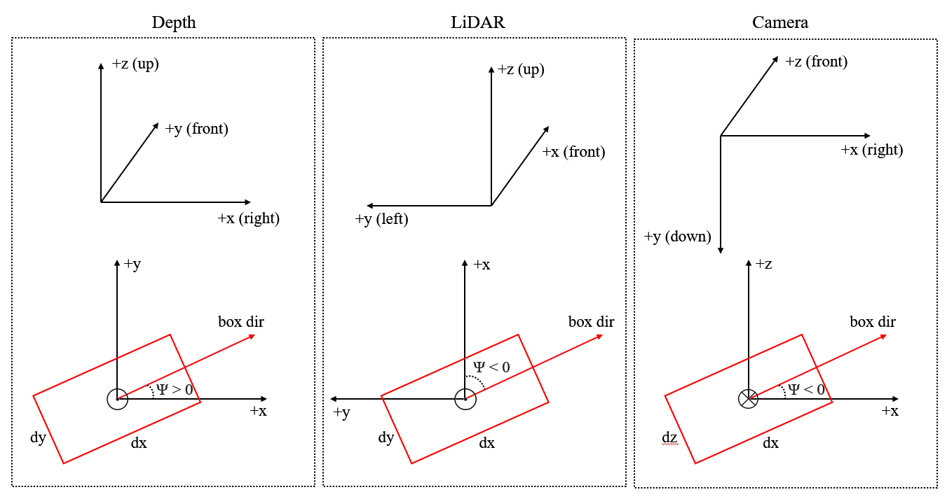
The three figures above are the 3D coordinate systems while the three figures below are the bird’s eye view.
We will stick to the three coordinate systems defined in this tutorial in the future.
Definition of the yaw angle
Please refer to wikipedia for the standard definition of the yaw angle. In object detection, we choose an axis as the gravity axis, and a reference direction on the plane \(\Pi\) perpendicular to the gravity axis, then the reference direction has a yaw angle of 0, and other directions on \(\Pi\) have non-zero yaw angles depending on its angle with the reference direction.
Currently, for all supported datasets, annotations do not include pitch angle and roll angle, which means we need only consider the yaw angle when predicting boxes and calculating overlap between boxes.
In MMDetection3D, all three coordinate systems are right-handed coordinate systems, which means the ascending direction of the yaw angle is counter-clockwise if viewed from the negative direction of the gravity axis (the axis is pointing at one’s eyes).
The figure below shows that, in this right-handed coordinate system, if we set the positive direction of the x-axis as a reference direction, then the positive direction of the y-axis has a yaw angle of \(\frac{\pi}{2}\).
                     z up  y front (yaw=0.5*pi)
                      ^    ^
                      |   /
                      |  /
                      | /
                      |/
left (yaw=pi)  ------ 0 ------> x right (yaw=0)
For a box, the value of its yaw angle equals its direction minus a reference direction. In all three coordinate systems in MMDetection3D, the reference direction is always the positive direction of the x-axis, while the direction of a box is defined to be parallel with the x-axis if its yaw angle is 0. The definition of the yaw angle of a box is illustrated in the figure below.
y front
  ^      box direction (yaw=0.5*pi)
 /|\        ^
  |        /|\
  |     ____|____
  |    |    |    |
  |    |    |    |
__|____|____|____|______\ x right
  |    |    |    |      /
  |    |    |    |
  |    |____|____|
  |
Definition of the box dimensions
The definition of the box dimensions cannot be disentangled with the definition of the yaw angle. In the previous section, we said that the direction of a box is defined to be parallel with the x-axis if its yaw angle is 0. Then naturally, the dimension of a box which corresponds to the x-axis should be \(dx\). However, this is not always the case in some datasets (we will address that later).
The following figures show the meaning of the correspondence between the x-axis and \(dx\), and between the y-axis and \(dy\).
y front
  ^      box direction (yaw=0.5*pi)
 /|\        ^
  |        /|\
  |     ____|____
  |    |    |    |
  |    |    |    | dx
__|____|____|____|______\ x right
  |    |    |    |      /
  |    |    |    |
  |    |____|____|
  |         dy
Note that the box direction is always parallel with the edge \(dx\).
y front
  ^     _________
 /|\   |    |    |
  |    |    |    |
  |    |    |    | dy
  |    |____|____|____\  box direction (yaw=0)
  |    |    |    |    /
__|____|____|____|_________\ x right
  |    |    |    |         /
  |    |____|____|
  |         dx
  |
Relation with raw coordinate systems of supported datasets
KITTI
The raw annotation of KITTI is under camera coordinate system, see get_label_anno. In MMDetection3D, to train LiDAR-based models on KITTI, the data is first converted from camera coordinate system to LiDAR coordinate system, see get_ann_info. For training vision-based models, the data is kept in the camera coordinate system.
In SECOND, the LiDAR coordinate system for a box is defined as follows (a bird’s eye view):
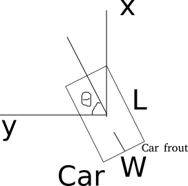
For each box, the dimensions are \((w, l, h)\), and the reference direction for the yaw angle is the positive direction of the y axis. For more details, refer to the repo.
Our LiDAR coordinate system has two changes:
The yaw angle is defined to be right-handed instead of left-handed for consistency;
The box dimensions are \((l, w, h)\) instead of \((w, l, h)\), since \(w\) corresponds to \(dy\) and \(l\) corresponds to \(dx\) in KITTI.
Waymo
We use the KITTI-format data of Waymo dataset. Therefore, KITTI and Waymo also share the same coordinate system in our implementation.
NuScenes
NuScenes provides a toolkit for evaluation, in which each box is wrapped into a Box instance. The coordinate system of Box is different from our LiDAR coordinate system in that the first two elements of the box dimension correspond to \((dy, dx)\), or \((w, l)\), respectively, instead of the reverse. For more details, please refer to the NuScenes tutorial.
Readers may refer to the NuScenes development kit for the definition of a NuScenes box and implementation of NuScenes evaluation.
Lyft
Lyft shares the same data format with NuScenes as far as coordinate system is involved.
Please refer to the official website for more information.
ScanNet
The raw data of ScanNet is not point cloud but mesh. The sampled point cloud data is under our depth coordinate system. For ScanNet detection task, the box annotations are axis-aligned, and the yaw angle is always zero. Therefore the direction of the yaw angle in our depth coordinate system makes no difference regarding ScanNet.
SUN RGB-D
The raw data of SUN RGB-D is not point cloud but RGB-D image. By back projection, we obtain the corresponding point cloud for each image, which is under our Depth coordinate system. However, the annotation is not under our system and thus needs conversion.
For the conversion from raw annotation to annotation under our Depth coordinate system, please refer to sunrgbd_data_utils.py.
S3DIS
S3DIS shares the same coordinate system as ScanNet in our implementation. However, S3DIS is a segmentation-task-only dataset, and thus no annotation is coordinate system sensitive.
Examples
Box conversion (between different coordinate systems)
Take the conversion between our Camera coordinate system and LiDAR coordinate system as an example:
First, for points and box centers, the coordinates before and after the conversion satisfy the following relationship:
\(x_{LiDAR}=z_{camera}\)
\(y_{LiDAR}=-x_{camera}\)
\(z_{LiDAR}=-y_{camera}\)
Then, the box dimensions before and after the conversion satisfy the following relationship:
\(dx_{LiDAR}=dx_{camera}\)
\(dy_{LiDAR}=dz_{camera}\)
\(dz_{LiDAR}=dy_{camera}\)
Finally, the yaw angle should also be converted:
\(r_{LiDAR}=-\frac{\pi}{2}-r_{camera}\)
See the code here for more details.
Bird’s Eye View
The BEV of a camera coordinate system box is \((x, z, dx, dz, -r)\) if the 3D box is \((x, y, z, dx, dy, dz, r)\). The inversion of the sign of the yaw angle is because the positive direction of the gravity axis of the Camera coordinate system points to the ground.
See the code here for more details.
Common FAQ
Q2: In every coordinate system, do the three axes point exactly to the right, the front, and the ground, respectively?
No. For example, in KITTI, we need a calibration matrix when converting from Camera coordinate system to LiDAR coordinate system.
Q3: How does a phase difference of \(2\pi\) in the yaw angle of a box affect evaluation?
For IoU calculation, a phase difference of \(2\pi\) in the yaw angle will result in the same box, thus not affecting evaluation.
For angle prediction evaluation such as the NDS metric in NuScenes and the AOS metric in KITTI, the angle of predicted boxes will be first standardized, so the phase difference of \(2\pi\) will not change the result.
Q4: How does a phase difference of \(\pi\) in the yaw angle of a box affect evaluation?
For IoU calculation, a phase difference of \(\pi\) in the yaw angle will result in the same box, thus not affecting evaluation.
However, for angle prediction evaluation, this will result in the exact opposite direction.
Just think about a car. The yaw angle is the angle between the direction of the car front and the positive direction of the x-axis. If we add \(\pi\) to this angle, the car front will become the car rear.
For categories such as barrier, the front and the rear have no difference, therefore a phase difference of \(\pi\) will not affect the angle prediction score.
Tutorial 7: Backends Support
We support different file client backends: Disk, Ceph and LMDB, etc. Here is an example of how to modify configs for Ceph-based data loading and saving.
Load data and annotations from Ceph
We support loading data and generated annotation info files (pkl and json) from Ceph:
# set file client backends as Ceph
file_client_args = dict(
    backend='petrel',
    path_mapping=dict({
        './data/nuscenes/':
        's3://openmmlab/datasets/detection3d/nuscenes/', # replace the path with your data path on Ceph
        'data/nuscenes/':
        's3://openmmlab/datasets/detection3d/nuscenes/' # replace the path with your data path on Ceph
    }))

db_sampler = dict(
    data_root=data_root,
    info_path=data_root + 'kitti_dbinfos_train.pkl',
    rate=1.0,
    prepare=dict(filter_by_difficulty=[-1], filter_by_min_points=dict(Car=5)),
    sample_groups=dict(Car=15),
    classes=class_names,
    # set file client for points loader to load training data
    points_loader=dict(
        type='LoadPointsFromFile',
        coord_type='LIDAR',
        load_dim=4,
        use_dim=4,
        file_client_args=file_client_args),
    # set file client for data base sampler to load db info file
    file_client_args=file_client_args)

train_pipeline = [
    # set file client for loading training data
    dict(type='LoadPointsFromFile', coord_type='LIDAR', load_dim=4, use_dim=4, file_client_args=file_client_args),
    # set file client for loading training data annotations
    dict(type='LoadAnnotations3D', with_bbox_3d=True, with_label_3d=True, file_client_args=file_client_args),
    dict(type='ObjectSample', db_sampler=db_sampler),
    dict(
        type='ObjectNoise',
        num_try=100,
        translation_std=[0.25, 0.25, 0.25],
        global_rot_range=[0.0, 0.0],
        rot_range=[-0.15707963267, 0.15707963267]),
    dict(type='RandomFlip3D', flip_ratio_bev_horizontal=0.5),
    dict(
        type='GlobalRotScaleTrans',
        rot_range=[-0.78539816, 0.78539816],
        scale_ratio_range=[0.95, 1.05]),
    dict(type='PointsRangeFilter', point_cloud_range=point_cloud_range),
    dict(type='ObjectRangeFilter', point_cloud_range=point_cloud_range),
    dict(type='PointShuffle'),
    dict(type='DefaultFormatBundle3D', class_names=class_names),
    dict(type='Collect3D', keys=['points', 'gt_bboxes_3d', 'gt_labels_3d'])
]
test_pipeline = [
    # set file client for loading validation/testing data
    dict(type='LoadPointsFromFile', coord_type='LIDAR', load_dim=4, use_dim=4, file_client_args=file_client_args),
    dict(
        type='MultiScaleFlipAug3D',
        img_scale=(1333, 800),
        pts_scale_ratio=1,
        flip=False,
        transforms=[
            dict(
                type='GlobalRotScaleTrans',
                rot_range=[0, 0],
                scale_ratio_range=[1., 1.],
                translation_std=[0, 0, 0]),
            dict(type='RandomFlip3D'),
            dict(
                type='PointsRangeFilter', point_cloud_range=point_cloud_range),
            dict(
                type='DefaultFormatBundle3D',
                class_names=class_names,
                with_label=False),
            dict(type='Collect3D', keys=['points'])
        ])
]

data = dict(
    # set file client for loading training info files (.pkl)
    train=dict(
        type='RepeatDataset',
        times=2,
        dataset=dict(pipeline=train_pipeline, classes=class_names, file_client_args=file_client_args)),
    # set file client for loading validation info files (.pkl)
    val=dict(pipeline=test_pipeline, classes=class_names,file_client_args=file_client_args),
    # set file client for loading testing info files (.pkl)
    test=dict(pipeline=test_pipeline, classes=class_names, file_client_args=file_client_args))
Load pretrained model from Ceph
model = dict(
    pts_backbone=dict(
        _delete_=True,
        type='NoStemRegNet',
        arch='regnetx_1.6gf',
        init_cfg=dict(
            type='Pretrained', checkpoint='s3://openmmlab/checkpoints/mmdetection3d/regnetx_1.6gf'), # replace the path with your pretrained model path on Ceph
        ...
Load checkpoint from Ceph
# replace the path with your checkpoint path on Ceph
load_from = 's3://openmmlab/checkpoints/mmdetection3d/v0.1.0_models/pointpillars/hv_pointpillars_secfpn_6x8_160e_kitti-3d-car/hv_pointpillars_secfpn_6x8_160e_kitti-3d-car_20200620_230614-77663cd6.pth.pth'
resume_from = None
workflow = [('train', 1)]
Save checkpoint into Ceph
# checkpoint saving
# replace the path with your checkpoint saving path on Ceph
checkpoint_config = dict(interval=1, max_keep_ckpts=2, out_dir='s3://openmmlab/mmdetection3d')
EvalHook saves the best checkpoint into Ceph
# replace the path with your checkpoint saving path on Ceph
evaluation = dict(interval=1, save_best='bbox', out_dir='s3://openmmlab/mmdetection3d')
Save the training log into Ceph
The training log will be backed up to the specified Ceph path after training.
log_config = dict(
    interval=50,
    hooks=[
        dict(type='TextLoggerHook', out_dir='s3://openmmlab/mmdetection3d'),
    ])
You can also delete the local training log after backing up to the specified Ceph path by setting keep_local = False.
log_config = dict(
    interval=50,
    hooks=[
        dict(type='TextLoggerHook', out_dir='s3://openmmlab/mmdetection3d'', keep_local=False),
    ])
We provide lots of useful tools under tools/ directory.
Log Analysis
You can plot loss/mAP curves given a training log file. Run pip install seaborn first to install the dependency.
 loss curve image
python tools/analysis_tools/analyze_logs.py plot_curve [--keys ${KEYS}] [--title ${TITLE}] [--legend ${LEGEND}] [--backend ${BACKEND}] [--style ${STYLE}] [--out ${OUT_FILE}] [--mode ${MODE}] [--interval ${INTERVAL}]
Notice: If the metric you want to plot is calculated in the eval stage, you need to add the flag --mode eval. If you perform evaluation with an interval of ${INTERVAL}, you need to add the args --interval ${INTERVAL}.
Examples:
Plot the classification loss of some run.
python tools/analysis_tools/analyze_logs.py plot_curve log.json --keys loss_cls --legend loss_cls
Plot the classification and regression loss of some run, and save the figure to a pdf.
python tools/analysis_tools/analyze_logs.py plot_curve log.json --keys loss_cls loss_bbox --out losses.pdf
Compare the bbox mAP of two runs in the same figure.
# evaluate PartA2 and second on KITTI according to Car_3D_moderate_strict
python tools/analysis_tools/analyze_logs.py plot_curve tools/logs/PartA2.log.json tools/logs/second.log.json --keys KITTI/Car_3D_moderate_strict --legend PartA2 second --mode eval --interval 1
# evaluate PointPillars for car and 3 classes on KITTI according to Car_3D_moderate_strict
python tools/analysis_tools/analyze_logs.py plot_curve tools/logs/pp-3class.log.json tools/logs/pp.log.json --keys KITTI/Car_3D_moderate_strict --legend pp-3class pp --mode eval --interval 2
You can also compute the average training speed.
python tools/analysis_tools/analyze_logs.py cal_train_time log.json [--include-outliers]
The output is expected to be like the following.
-----Analyze train time of work_dirs/some_exp/20190611_192040.log.json-----
slowest epoch 11, average time is 1.2024
fastest epoch 1, average time is 1.1909
time std over epochs is 0.0028
average iter time: 1.1959 s/iter
Visualization
Results
To see the prediction results of trained models, you can run the following command
python tools/test.py ${CONFIG_FILE} ${CKPT_PATH} --show --show-dir ${SHOW_DIR}
After running this command, plotted results including input data and the output of networks visualized on the input (e.g. ***_points.obj and ***_pred.obj in single-modality 3D detection task) will be saved in ${SHOW_DIR}.
To see the prediction results during evaluation, you can run the following command
python tools/test.py ${CONFIG_FILE} ${CKPT_PATH} --eval 'mAP' --eval-options 'show=True' 'out_dir=${SHOW_DIR}'
After running this command, you will obtain the input data, the output of networks and ground-truth labels visualized on the input (e.g. ***_points.obj, ***_pred.obj, ***_gt.obj, ***_img.png and ***_pred.png in multi-modality detection task) in ${SHOW_DIR}. When show is enabled, Open3D will be used to visualize the results online. If you are running test in remote server without GUI, the online visualization is not supported, you can set show=False to only save the output results in {SHOW_DIR}.
As for offline visualization, you will have two options.
To visualize the results with Open3D backend, you can run the following command
python tools/misc/visualize_results.py ${CONFIG_FILE} --result ${RESULTS_PATH} --show-dir ${SHOW_DIR}

Or you can use 3D visualization software such as the MeshLab to open these files under ${SHOW_DIR} to see the 3D detection output. Specifically, open ***_points.obj to see the input point cloud and open ***_pred.obj to see the predicted 3D bounding boxes. This allows the inference and results generation to be done in remote server and the users can open them on their host with GUI.
Notice: The visualization API is a little unstable since we plan to refactor these parts together with MMDetection in the future.
Dataset
We also provide scripts to visualize the dataset without inference. You can use tools/misc/browse_dataset.py to show loaded data and ground-truth online and save them on the disk. Currently we support single-modality 3D detection and 3D segmentation on all the datasets, multi-modality 3D detection on KITTI and SUN RGB-D, as well as monocular 3D detection on nuScenes. To browse the KITTI dataset, you can run the following command
python tools/misc/browse_dataset.py configs/_base_/datasets/kitti-3d-3class.py --task det --output-dir ${OUTPUT_DIR} --online
Notice: Once specifying --output-dir, the images of views specified by users will be saved when pressing _ESC_ in open3d window. If you don’t have a monitor, you can remove the --online flag to only save the visualization results and browse them offline.
To verify the data consistency and the effect of data augmentation, you can also add --aug flag to visualize the data after data augmentation using the command as below:
python tools/misc/browse_dataset.py configs/_base_/datasets/kitti-3d-3class.py --task det --aug --output-dir ${OUTPUT_DIR} --online
If you also want to show 2D images with 3D bounding boxes projected onto them, you need to find a config that supports multi-modality data loading, and then change the --task args to multi_modality-det. An example is showed below
python tools/misc/browse_dataset.py configs/mvxnet/dv_mvx-fpn_second_secfpn_adamw_2x8_80e_kitti-3d-3class.py --task multi_modality-det --output-dir ${OUTPUT_DIR} --online

You can simply browse different datasets using different configs, e.g. visualizing the ScanNet dataset in 3D semantic segmentation task
python tools/misc/browse_dataset.py configs/_base_/datasets/scannet_seg-3d-20class.py --task seg --output-dir ${OUTPUT_DIR} --online

And browsing the nuScenes dataset in monocular 3D detection task
python tools/misc/browse_dataset.py configs/_base_/datasets/nus-mono3d.py --task mono-det --output-dir ${OUTPUT_DIR} --online

Model Serving
Note: This tool is still experimental now, only SECOND is supported to be served with TorchServe. We’ll support more models in the future.
In order to serve an MMDetection3D model with TorchServe, you can follow the steps:
1. Convert the model from MMDetection3D to TorchServe
python tools/deployment/mmdet3d2torchserve.py ${CONFIG_FILE} ${CHECKPOINT_FILE} \
--output-folder ${MODEL_STORE} \
--model-name ${MODEL_NAME}
Note: ${MODEL_STORE} needs to be an absolute path to a folder.
2. Build mmdet3d-serve docker image
docker build -t mmdet3d-serve:latest docker/serve/
3. Run mmdet3d-serve
Check the official docs for running TorchServe with docker.
In order to run it on the GPU, you need to install nvidia-docker. You can omit the --gpus argument in order to run on the CPU.
Example:
docker run --rm \
--cpus 8 \
--gpus device=0 \
-p8080:8080 -p8081:8081 -p8082:8082 \
--mount type=bind,source=$MODEL_STORE,target=/home/model-server/model-store \
mmdet3d-serve:latest
Read the docs about the Inference (8080), Management (8081) and Metrics (8082) APis
4. Test deployment
You can use test_torchserver.py to compare result of torchserver and pytorch.
python tools/deployment/test_torchserver.py ${IMAGE_FILE} ${CONFIG_FILE} ${CHECKPOINT_FILE} ${MODEL_NAME}
[--inference-addr ${INFERENCE_ADDR}] [--device ${DEVICE}] [--score-thr ${SCORE_THR}]
Example:
python tools/deployment/test_torchserver.py demo/data/kitti/kitti_000008.bin configs/second/hv_second_secfpn_6x8_80e_kitti-3d-car.py checkpoints/hv_second_secfpn_6x8_80e_kitti-3d-car_20200620_230238-393f000c.pth second
Model Complexity
You can use tools/analysis_tools/get_flops.py in MMDetection3D, a script adapted from flops-counter.pytorch, to compute the FLOPs and params of a given model.
python tools/analysis_tools/get_flops.py ${CONFIG_FILE} [--shape ${INPUT_SHAPE}]
You will get the results like this.
==============================
Input shape: (40000, 4)
Flops: 5.78 GFLOPs
Params: 953.83 k
==============================
Note: This tool is still experimental and we do not guarantee that the number is absolutely correct. You may well use the result for simple comparisons, but double check it before you adopt it in technical reports or papers.
FLOPs are related to the input shape while parameters are not. The default input shape is (1, 40000, 4).
Some operators are not counted into FLOPs like GN and custom operators. Refer to
mmcv.cnn.get_model_complexity_info()for details.We currently only support FLOPs calculation of single-stage models with single-modality input (point cloud or image). We will support two-stage and multi-modality models in the future.
Model Conversion
RegNet model to MMDetection
tools/model_converters/regnet2mmdet.py convert keys in pycls pretrained RegNet models to
MMDetection style.
python tools/model_converters/regnet2mmdet.py ${SRC} ${DST} [-h]
Detectron ResNet to Pytorch
tools/detectron2pytorch.py in MMDetection could convert keys in the original detectron pretrained
ResNet models to PyTorch style.
python tools/detectron2pytorch.py ${SRC} ${DST} ${DEPTH} [-h]
Prepare a model for publishing
tools/model_converters/publish_model.py helps users to prepare their model for publishing.
Before you upload a model to AWS, you may want to
convert model weights to CPU tensors
delete the optimizer states and
compute the hash of the checkpoint file and append the hash id to the filename.
python tools/model_converters/publish_model.py ${INPUT_FILENAME} ${OUTPUT_FILENAME}
E.g.,
python tools/model_converters/publish_model.py work_dirs/faster_rcnn/latest.pth faster_rcnn_r50_fpn_1x_20190801.pth
The final output filename will be faster_rcnn_r50_fpn_1x_20190801-{hash id}.pth.
Dataset Conversion
tools/data_converter/ contains tools for converting datasets to other formats. Most of them convert datasets to pickle based info files, like kitti, nuscenes and lyft. Waymo converter is used to reorganize waymo raw data like KITTI style. Users could refer to them for our approach to converting data format. It is also convenient to modify them to use as scripts like nuImages converter.
To convert the nuImages dataset into COCO format, please use the command below:
python -u tools/data_converter/nuimage_converter.py --data-root ${DATA_ROOT} --version ${VERSIONS} \
                                                    --out-dir ${OUT_DIR} --nproc ${NUM_WORKERS} --extra-tag ${TAG}
--data-root: the root of the dataset, defaults to./data/nuimages.--version: the version of the dataset, defaults tov1.0-mini. To get the full dataset, please use--version v1.0-train v1.0-val v1.0-mini--out-dir: the output directory of annotations and semantic masks, defaults to./data/nuimages/annotations/.--nproc: number of workers for data preparation, defaults to4. Larger number could reduce the preparation time as images are processed in parallel.--extra-tag: extra tag of the annotations, defaults tonuimages. This can be used to separate different annotations processed in different time for study.
More details could be referred to the doc for dataset preparation and README for nuImages dataset.
Benchmarks
Here we benchmark the training and testing speed of models in MMDetection3D, with some other open source 3D detection codebases.
Settings
Hardwares: 8 NVIDIA Tesla V100 (32G) GPUs, Intel(R) Xeon(R) Gold 6148 CPU @ 2.40GHz
Software: Python 3.7, CUDA 10.1, cuDNN 7.6.5, PyTorch 1.3, numba 0.48.0.
Model: Since all the other codebases implements different models, we compare the corresponding models including SECOND, PointPillars, Part-A2, and VoteNet with them separately.
Metrics: We use the average throughput in iterations of the entire training run and skip the first 50 iterations of each epoch to skip GPU warmup time.
Main Results
We compare the training speed (samples/s) with other codebases if they implement the similar models. The results are as below, the greater the numbers in the table, the faster of the training process. The models that are not supported by other codebases are marked by ×.
| Methods | MMDetection3D | OpenPCDet | votenet | Det3D |
|---|---|---|---|---|
| VoteNet | 358 | × | 77 | × |
| PointPillars-car | 141 | × | × | 140 |
| PointPillars-3class | 107 | 44 | × | × |
| SECOND | 40 | 30 | × | × |
| Part-A2 | 17 | 14 | × | × |
Details of Comparison
Modification for Calculating Speed
MMDetection3D: We try to use as similar settings as those of other codebases as possible using benchmark configs.
Det3D: For comparison with Det3D, we use the commit 519251e.
OpenPCDet: For comparison with OpenPCDet, we use the commit b32fbddb.
For training speed, we add code to record the running time in the file
./tools/train_utils/train_utils.py. We calculate the speed of each epoch, and report the average speed of all the epochs.(diff to make it use the same method for benchmarking speed - click to expand)
diff --git a/tools/train_utils/train_utils.py b/tools/train_utils/train_utils.py
index 91f21dd..021359d 100644
--- a/tools/train_utils/train_utils.py
+++ b/tools/train_utils/train_utils.py
@@ -2,6 +2,7 @@ import torch
 import os
 import glob
 import tqdm
+import datetime
 from torch.nn.utils import clip_grad_norm_


@@ -13,7 +14,10 @@ def train_one_epoch(model, optimizer, train_loader, model_func, lr_scheduler, ac
     if rank == 0:
         pbar = tqdm.tqdm(total=total_it_each_epoch, leave=leave_pbar, desc='train', dynamic_ncols=True)

+    start_time = None
     for cur_it in range(total_it_each_epoch):
+        if cur_it > 49 and start_time is None:
+            start_time = datetime.datetime.now()
         try:
             batch = next(dataloader_iter)
         except StopIteration:
@@ -55,9 +59,11 @@ def train_one_epoch(model, optimizer, train_loader, model_func, lr_scheduler, ac
                 tb_log.add_scalar('learning_rate', cur_lr, accumulated_iter)
                 for key, val in tb_dict.items():
                     tb_log.add_scalar('train_' + key, val, accumulated_iter)
+    endtime = datetime.datetime.now()
+    speed = (endtime - start_time).seconds / (total_it_each_epoch - 50)
     if rank == 0:
         pbar.close()
-    return accumulated_iter
+    return accumulated_iter, speed


 def train_model(model, optimizer, train_loader, model_func, lr_scheduler, optim_cfg,
@@ -65,6 +71,7 @@ def train_model(model, optimizer, train_loader, model_func, lr_scheduler, optim_
                 lr_warmup_scheduler=None, ckpt_save_interval=1, max_ckpt_save_num=50,
                 merge_all_iters_to_one_epoch=False):
     accumulated_iter = start_iter
+    speeds = []
     with tqdm.trange(start_epoch, total_epochs, desc='epochs', dynamic_ncols=True, leave=(rank == 0)) as tbar:
         total_it_each_epoch = len(train_loader)
         if merge_all_iters_to_one_epoch:
@@ -82,7 +89,7 @@ def train_model(model, optimizer, train_loader, model_func, lr_scheduler, optim_
                 cur_scheduler = lr_warmup_scheduler
             else:
                 cur_scheduler = lr_scheduler
-            accumulated_iter = train_one_epoch(
+            accumulated_iter, speed = train_one_epoch(
                 model, optimizer, train_loader, model_func,
                 lr_scheduler=cur_scheduler,
                 accumulated_iter=accumulated_iter, optim_cfg=optim_cfg,
@@ -91,7 +98,7 @@ def train_model(model, optimizer, train_loader, model_func, lr_scheduler, optim_
                 total_it_each_epoch=total_it_each_epoch,
                 dataloader_iter=dataloader_iter
             )
-
+            speeds.append(speed)
             # save trained model
             trained_epoch = cur_epoch + 1
             if trained_epoch % ckpt_save_interval == 0 and rank == 0:
@@ -107,6 +114,8 @@ def train_model(model, optimizer, train_loader, model_func, lr_scheduler, optim_
                 save_checkpoint(
                     checkpoint_state(model, optimizer, trained_epoch, accumulated_iter), filename=ckpt_name,
                 )
+            print(speed)
+    print(f'*******{sum(speeds) / len(speeds)}******')


 def model_state_to_cpu(model_state):
VoteNet
MMDetection3D: With release v0.1.0, run
./tools/dist_train.sh configs/votenet/votenet_16x8_sunrgbd-3d-10class.py 8 --no-validatevotenet: At commit 2f6d6d3, run
python train.py --dataset sunrgbd --batch_size 16Then benchmark the test speed by running
python eval.py --dataset sunrgbd --checkpoint_path log_sunrgbd/checkpoint.tar --batch_size 1 --dump_dir eval_sunrgbd --cluster_sampling seed_fps --use_3d_nms --use_cls_nms --per_class_proposalNote that eval.py is modified to compute inference time.
(diff to benchmark the similar models - click to expand)
diff --git a/eval.py b/eval.py
  index c0b2886..04921e9 100644
  --- a/eval.py
  +++ b/eval.py
  @@ -10,6 +10,7 @@ import os
   import sys
   import numpy as np
   from datetime import datetime
  +import time
   import argparse
   import importlib
   import torch
  @@ -28,7 +29,7 @@ parser.add_argument('--checkpoint_path', default=None, help='Model checkpoint pa
   parser.add_argument('--dump_dir', default=None, help='Dump dir to save sample outputs [default: None]')
   parser.add_argument('--num_point', type=int, default=20000, help='Point Number [default: 20000]')
   parser.add_argument('--num_target', type=int, default=256, help='Point Number [default: 256]')
  -parser.add_argument('--batch_size', type=int, default=8, help='Batch Size during training [default: 8]')
  +parser.add_argument('--batch_size', type=int, default=1, help='Batch Size during training [default: 8]')
   parser.add_argument('--vote_factor', type=int, default=1, help='Number of votes generated from each seed [default: 1]')
   parser.add_argument('--cluster_sampling', default='vote_fps', help='Sampling strategy for vote clusters: vote_fps, seed_fps, random [default: vote_fps]')
   parser.add_argument('--ap_iou_thresholds', default='0.25,0.5', help='A list of AP IoU thresholds [default: 0.25,0.5]')
  @@ -132,6 +133,7 @@ CONFIG_DICT = {'remove_empty_box': (not FLAGS.faster_eval), 'use_3d_nms': FLAGS.
   # ------------------------------------------------------------------------- GLOBAL CONFIG END

   def evaluate_one_epoch():
  +    time_list = list()
       stat_dict = {}
       ap_calculator_list = [APCalculator(iou_thresh, DATASET_CONFIG.class2type) \
           for iou_thresh in AP_IOU_THRESHOLDS]
  @@ -144,6 +146,8 @@ def evaluate_one_epoch():

           # Forward pass
           inputs = {'point_clouds': batch_data_label['point_clouds']}
  +        torch.cuda.synchronize()
  +        start_time = time.perf_counter()
           with torch.no_grad():
               end_points = net(inputs)

  @@ -161,6 +165,12 @@ def evaluate_one_epoch():

           batch_pred_map_cls = parse_predictions(end_points, CONFIG_DICT)
           batch_gt_map_cls = parse_groundtruths(end_points, CONFIG_DICT)
  +        torch.cuda.synchronize()
  +        elapsed = time.perf_counter() - start_time
  +        time_list.append(elapsed)
  +
  +        if len(time_list==200):
  +            print("average inference time: %4f"%(sum(time_list[5:])/len(time_list[5:])))
           for ap_calculator in ap_calculator_list:
               ap_calculator.step(batch_pred_map_cls, batch_gt_map_cls)
PointPillars-car
MMDetection3D: With release v0.1.0, run
./tools/dist_train.sh configs/benchmark/hv_pointpillars_secfpn_3x8_100e_det3d_kitti-3d-car.py 8 --no-validateDet3D: At commit 519251e, use
kitti_point_pillars_mghead_syncbn.pyand run./tools/scripts/train.sh --launcher=slurm --gpus=8
Note that the config in train.sh is modified to train point pillars.
(diff to benchmark the similar models - click to expand)
diff --git a/tools/scripts/train.sh b/tools/scripts/train.sh
index 3a93f95..461e0ea 100755
--- a/tools/scripts/train.sh
+++ b/tools/scripts/train.sh
@@ -16,9 +16,9 @@ then
 fi

 # Voxelnet
-python -m torch.distributed.launch --nproc_per_node=8 ./tools/train.py examples/second/configs/  kitti_car_vfev3_spmiddlefhd_rpn1_mghead_syncbn.py --work_dir=$SECOND_WORK_DIR
+# python -m torch.distributed.launch --nproc_per_node=8 ./tools/train.py examples/second/configs/  kitti_car_vfev3_spmiddlefhd_rpn1_mghead_syncbn.py --work_dir=$SECOND_WORK_DIR
 # python -m torch.distributed.launch --nproc_per_node=8 ./tools/train.py examples/cbgs/configs/  nusc_all_vfev3_spmiddleresnetfhd_rpn2_mghead_syncbn.py --work_dir=$NUSC_CBGS_WORK_DIR
 # python -m torch.distributed.launch --nproc_per_node=8 ./tools/train.py examples/second/configs/  lyft_all_vfev3_spmiddleresnetfhd_rpn2_mghead_syncbn.py --work_dir=$LYFT_CBGS_WORK_DIR

 # PointPillars
-# python -m torch.distributed.launch --nproc_per_node=8 ./tools/train.py ./examples/point_pillars/configs/  original_pp_mghead_syncbn_kitti.py --work_dir=$PP_WORK_DIR
+python -m torch.distributed.launch --nproc_per_node=8 ./tools/train.py ./examples/point_pillars/configs/  kitti_point_pillars_mghead_syncbn.py
PointPillars-3class
MMDetection3D: With release v0.1.0, run
./tools/dist_train.sh configs/benchmark/hv_pointpillars_secfpn_4x8_80e_pcdet_kitti-3d-3class.py 8 --no-validateOpenPCDet: At commit b32fbddb, run
cd tools
sh scripts/slurm_train.sh ${PARTITION} ${JOB_NAME} 8  --cfg_file ./cfgs/kitti_models/pointpillar.yaml --batch_size 32  --workers 32 --epochs 80
SECOND
For SECOND, we mean the SECONDv1.5 that was first implemented in second.Pytorch. Det3D’s implementation of SECOND uses its self-implemented Multi-Group Head, so its speed is not compatible with other codebases.
MMDetection3D: With release v0.1.0, run
./tools/dist_train.sh configs/benchmark/hv_second_secfpn_4x8_80e_pcdet_kitti-3d-3class.py 8 --no-validateOpenPCDet: At commit b32fbddb, run
cd tools
sh ./scripts/slurm_train.sh ${PARTITION} ${JOB_NAME} 8  --cfg_file ./cfgs/kitti_models/second.yaml --batch_size 32  --workers 32 --epochs 80
Part-A2
MMDetection3D: With release v0.1.0, run
./tools/dist_train.sh configs/benchmark/hv_PartA2_secfpn_4x8_cyclic_80e_pcdet_kitti-3d-3class.py 8 --no-validateOpenPCDet: At commit b32fbddb, train the model by running
cd tools
sh ./scripts/slurm_train.sh ${PARTITION} ${JOB_NAME} 8  --cfg_file ./cfgs/kitti_models/PartA2.yaml --batch_size 32 --workers 32 --epochs 80
FAQ
We list some potential troubles encountered by users and developers, along with their corresponding solutions. Feel free to enrich the list if you find any frequent issues and contribute your solutions to solve them. If you have any trouble with environment configuration, model training, etc, please create an issue using the provided templates and fill in all required information in the template.
MMCV/MMDet/MMDet3D Installation
If you faced the error shown below when importing open3d:
OSError: /lib/x86_64-linux-gnu/libm.so.6: version 'GLIBC_2.27' not foundplease downgrade open3d to 0.9.0.0, because the latest open3d needs the support of file ‘GLIBC_2.27’, which only exists in Ubuntu 18.04, not in Ubuntu 16.04.
If you faced the error when importing pycocotools, this is because nuscenes-devkit installs pycocotools but mmdet relies on mmpycocotools. The current workaround is as below. We will migrate to use pycocotools in the future.
pip uninstall pycocotools mmpycocotools
pip install mmpycocotools
NOTE: We have migrated to use pycocotools in mmdet3d >= 0.13.0.
If you face the error shown below when importing pycocotools:
ValueError: numpy.ndarray size changed, may indicate binary incompatibility. Expected 88 from C header, got 80 from PyObjectplease downgrade pycocotools to 2.0.1 because of the incompatibility between the newest pycocotools and numpy < 1.20.0. Or you can compile and install the latest pycocotools from source as below:
pip install -e "git+https://github.com/cocodataset/cocoapi#egg=pycocotools&subdirectory=PythonAPI"or
pip install -e "git+https://github.com/ppwwyyxx/cocoapi#egg=pycocotools&subdirectory=PythonAPI"
v1.0.0rc1
Operators Migration
We have adopted CUDA operators compiled from mmcv and removed all the CUDA operators in mmdet3d. We now do not need to compile the CUDA operators in mmdet3d anymore.
Waymo dataset converter refactoring
In this version we did a major code refactoring that boosted the performance of waymo dataset conversion by multiprocessing. Meanwhile, we also fixed the imprecise timestamps saving issue in waymo dataset conversion. This change introduces following backward compatibility breaks:
The point cloud .bin files of waymo dataset need to be regenerated. In the .bin files each point occupies 6
float32and the meaning of the lastfloat32now changed from imprecise timestamps to range frame offset. The range frame offset for each point is calculated asri * h * w + row * w + colif the point is from the TOP lidar or-1otherwise. Theh,wdenote the height and width of the TOP lidar’s range frame. Theri,row,coldenote the return index, the row and the column of the range frame where each point locates. Following tables show the difference across the change:
Before
| Element offset (float32) | 0 | 1 | 2 | 3 | 4 | 5 |
|---|---|---|---|---|---|---|
| Bytes offset | 0 | 4 | 8 | 12 | 16 | 20 |
| Meaning | x | y | z | intensity | elongation | imprecise timestamp |
After
| Element offset (float32) | 0 | 1 | 2 | 3 | 4 | 5 |
|---|---|---|---|---|---|---|
| Bytes offset | 0 | 4 | 8 | 12 | 16 | 20 |
| Meaning | x | y | z | intensity | elongation | range frame offset |
The objects’ point cloud .bin files in the GT-database of waymo dataset need to be regenerated because we also dumped the range frame offset for each point into it. Following tables show the difference across the change:
Before
| Element offset (float32) | 0 | 1 | 2 | 3 | 4 |
|---|---|---|---|---|---|
| Bytes offset | 0 | 4 | 8 | 12 | 16 |
| Meaning | x | y | z | intensity | elongation |
After
| Element offset (float32) | 0 | 1 | 2 | 3 | 4 | 5 |
|---|---|---|---|---|---|---|
| Bytes offset | 0 | 4 | 8 | 12 | 16 | 20 |
| Meaning | x | y | z | intensity | elongation | range frame offset |
Any configuration that uses waymo dataset with GT Augmentation should change the
db_sampler.points_loader.load_dimfrom5to6.
v1.0.0rc0
Coordinate system refactoring
In this version, we did a major code refactoring which improved the consistency among the three coordinate systems (and corresponding box representation), LiDAR, Camera, and Depth. A brief summary for this refactoring is as follows:
The three coordinate systems are all right-handed now (which means the yaw angle increases in the counterclockwise direction).
The LiDAR system
(x_size, y_size, z_size)corresponds to(l, w, h)instead of(w, l, h). This is more natural sincelis parallel with the direction where the yaw angle is zero, and we prefer using the positive direction of thexaxis as that direction, which is exactly how we define yaw angle in Depth and Camera coordinate systems.The APIs for box-related operations are improved and now are more user-friendly.
NOTICE!!
Since definitions of box representation have changed, the annotation data of most datasets require updating:
SUN RGB-D: Yaw angles in the annotation should be reversed.
KITTI: For LiDAR boxes in GT databases, (x_size, y_size, z_size, yaw) out of (x, y, z, x_size, y_size, z_size) should be converted from the old LiDAR coordinate system to the new one. The training/validation data annotations should be left unchanged since they are under the Camera coordinate system, which is unmodified after the refactoring.
Waymo: Same as KITTI.
nuScenes: For LiDAR boxes in training/validation data and GT databases, (x_size, y_size, z_size, yaw) out of (x, y, z, x_size, y_size, z_size) should be converted.
Lyft: Same as nuScenes.
Please regenerate the data annotation/GT database files or use update_data_coords.py to update the data.
To use boxes under Depth and LiDAR coordinate systems, or to convert boxes between different coordinate systems, users should be aware of the difference between the old and new definitions. For example, the rotation, flipping, and bev functions of DepthInstance3DBoxes and LiDARInstance3DBoxes and box conversion functions have all been reimplemented in the refactoring.
Consequently, functions like output_to_lyft_box undergo small modification to adapt to the new LiDAR/Depth box.
Since the LiDAR system (x_size, y_size, z_size) now corresponds to (l, w, h) instead of (w, l, h), the anchor sizes for LiDAR boxes are also changed, e.g., from [1.6, 3.9, 1.56] to [3.9, 1.6, 1.56].
Functions only involving points are generally unaffected except if they rely on some refactored utility functions such as rotation_3d_in_axis.
Other BC-breaking or new features:
array_converter: Please refer to array_converter.py. Functions wrapped witharray_convertercan convert array-like input types oftorch.Tensor,np.ndarray, andlist/tuple/floattotorch.Tensorto process in an unified PyTorch pipeline. The result may finally be converted back to the input type. Most functions in utils.py are wrapped witharray_converter.points_in_boxesandpoints_in_boxes_batchwill be deprecated soon. They are renamed topoints_in_boxes_partandpoints_in_boxes_allrespectively, with more detailed docstrings. The major difference of the two functions is that if a point is enclosed by multiple boxes,points_in_boxes_partwill only return the index of the first enclosing box whilepoints_in_boxes_allwill return all the indices of enclosing boxes.rotation_3d_in_axis: Please refer to utils.py. Now this function supports multiple input types and more options. The function with the same name in box_np_ops.py is deleted since we do not need another function to tackle with NumPy data.rotation_2d,points_cam2img, andlimit_periodin box_np_ops.py are also deleted for the same reason.bevmethod ofCameraInstance3DBoxes: Changed it to be consistent with the definition of bev in Depth and LiDAR coordinate systems.Data augmentation utils in data_augment_utils.py now follow the rules of a right-handed system.
We do not need the yaw hacking in KITTI anymore after refining
get_direction_target. Interested users may refer to PR #677 .
0.16.0
Returned values of QueryAndGroup operation
We modified the returned grouped_xyz value of operation QueryAndGroup to support PAConv segmentor. Originally, the grouped_xyz is centered by subtracting the grouping centers, which represents the relative positions of grouped points. Now, we didn’t perform such subtraction and the returned grouped_xyz stands for the absolute coordinates of these points.
Note that, the other returned variables of QueryAndGroup such as new_features, unique_cnt and grouped_idx are not affected.
NuScenes coco-style data pre-processing
We remove the rotation and dimension hack in the monocular 3D detection on nuScenes. Specifically, we transform the rotation and dimension of boxes defined by nuScenes devkit to the coordinate system of our CameraInstance3DBoxes in the pre-processing and transform them back in the post-processing. In this way, we can remove the corresponding hack used in the visualization tools. The modification also guarantees the correctness of all the operations based on our CameraInstance3DBoxes (such as NMS and flip augmentation) when training monocular 3D detectors.
The modification only influences nuScenes coco-style json files. Please re-run the nuScenes data preparation script if necessary. See more details in the PR #744.
ScanNet dataset for ImVoxelNet
We adopt a new pre-processing procedure for the ScanNet dataset in order to support ImVoxelNet, which is a multi-view method requiring image data. In previous versions of MMDetection3D, ScanNet dataset was only used for point cloud based 3D detection and segmentation methods. We plan adding ImVoxelNet to our model zoo, thus updating ScanNet correspondingly by adding image-related pre-processing steps. Specifically, we made these changes:
Add script for extracting RGB data.
Update script for annotation creating.
Add instructions in the documents on preparing image data.
Please refer to the ScanNet README.md for more details.
0.15.0
MMCV Version
In order to fix the problem that the priority of EvalHook is too low, all hook priorities have been re-adjusted in 1.3.8, so MMDetection 2.14.0 needs to rely on the latest MMCV 1.3.8 version. For related information, please refer to #1120, for related issues, please refer to #5343.
Unified parameter initialization
To unify the parameter initialization in OpenMMLab projects, MMCV supports BaseModule that accepts init_cfg to allow the modules’ parameters initialized in a flexible and unified manner. Now the users need to explicitly call model.init_weights() in the training script to initialize the model (as in here, previously this was handled by the detector. Please refer to PR #622 for details.
BackgroundPointsFilter
We modified the dataset augmentation function BackgroundPointsFilter(here). In previous version of MMdetection3D, BackgroundPointsFilter changes the gt_bboxes_3d’s bottom center to the gravity center. In MMDetection3D 0.15.0,
BackgroundPointsFilter will not change it. Please refer to PR #609 for details.
Enhance IndoorPatchPointSample transform
We enhance the pipeline function IndoorPatchPointSample used in point cloud segmentation task by adding more choices for patch selection. Also, we plan to remove the unused parameter sample_rate in the future. Please modify the code as well as the config files accordingly if you use this transform.
0.14.0
Dataset class for 3D segmentation task
We remove a useless parameter label_weight from segmentation datasets including Custom3DSegDataset, ScanNetSegDataset and S3DISSegDataset since this weight is utilized in the loss function of model class. Please modify the code as well as the config files accordingly if you use or inherit from these codes.
ScanNet data pre-processing
We adopt new pre-processing and conversion steps of ScanNet dataset. In previous versions of MMDetection3D, ScanNet dataset was only used for 3D detection task, where we trained on the training set and tested on the validation set. In MMDetection3D 0.14.0, we further support 3D segmentation task on ScanNet, which includes online benchmarking on test set. Since the alignment matrix is not provided for test set data, we abandon the alignment of points in data generation steps to support both tasks. Besides, as 3D segmentation requires per-point prediction, we also remove the down-sampling step in data generation.
In the new ScanNet processing scripts, we save the unaligned points for all the training, validation and test set. For train and val set with annotations, we also store the
axis_align_matrixin data infos. For ground-truth bounding boxes, we store boxes in both aligned and unaligned coordinates with keygt_boxes_upright_depthand keyunaligned_gt_boxes_upright_depthrespectively in data infos.In
ScanNetDataset, we now load theaxis_align_matrixas a part of data annotations. If it is not contained in old data infos, we will use identity matrix for compatibility. We also add a transform functionGlobalAlignmentin ScanNet detection data pipeline to align the points.Since the aligned boxes share the same key as in old data infos, we do not need to modify the code related to it. But do remember that they are not in the same coordinate system as the saved points.
There is an
PointSamplepipeline in the data pipelines for ScanNet detection task which down-samples points. So removing down-sampling in data generation will not affect the code.
We have trained a VoteNet model on the newly processed ScanNet dataset and get similar benchmark results. In order to prepare ScanNet data for both detection and segmentation tasks, please re-run the new pre-processing scripts following the ScanNet README.md.
0.12.0
SUNRGBD dataset for ImVoteNet
We adopt a new pre-processing procedure for the SUNRGBD dataset in order to support ImVoteNet, which is a multi-modality method requiring both image and point cloud data. In previous versions of MMDetection3D, SUNRGBD dataset was only used for point cloud based 3D detection methods. In MMDetection3D 0.12.0, we add ImVoteNet to our model zoo, thus updating SUNRGBD correspondingly by adding image-related pre-processing steps. Specifically, we made these changes:
Fix a bug in the image file path in meta data.
Convert calibration matrices from double to float to avoid type mismatch in further operations.
Add instructions in the documents on preparing image data.
Please refer to the SUNRGBD README.md for more details.
0.6.0
VoteNet and H3DNet model structure update
In MMDetection 0.6.0, we updated the model structures of VoteNet and H3DNet, therefore model checkpoints generated by MMDetection < 0.6.0 should be first converted to a format compatible with the latest structures via convert_votenet_checkpoints.py and convert_h3dnet_checkpoints.py . For more details, please refer to the VoteNet README.md and H3DNet README.md.
mmdet3d.datasets
mmdet3d.models
detectors
backbones
- class mmdet3d.models.backbones.DGCNNBackbone(in_channels, num_samples=(20, 20, 20), knn_modes=('D-KNN', 'F-KNN', 'F-KNN'), radius=(None, None, None), gf_channels=((64, 64), (64, 64), (64)), fa_channels=(1024), act_cfg={'type': 'ReLU'}, init_cfg=None)[source]
Backbone network for DGCNN.
- Parameters
in_channels (int) – Input channels of point cloud.
num_samples (tuple[int], optional) – The number of samples for knn or ball query in each graph feature (GF) module. Defaults to (20, 20, 20).
knn_modes (tuple[str], optional) – Mode of KNN of each knn module. Defaults to (‘D-KNN’, ‘F-KNN’, ‘F-KNN’).
radius (tuple[float], optional) – Sampling radii of each GF module. Defaults to (None, None, None).
gf_channels (tuple[tuple[int]], optional) – Out channels of each mlp in GF module. Defaults to ((64, 64), (64, 64), (64, )).
fa_channels (tuple[int], optional) – Out channels of each mlp in FA module. Defaults to (1024, ).
act_cfg (dict, optional) – Config of activation layer. Defaults to dict(type=’ReLU’).
init_cfg (dict, optional) – Initialization config. Defaults to None.
- forward(points)[source]
Forward pass.
- Parameters
points (torch.Tensor) – point coordinates with features, with shape (B, N, in_channels).
- Returns
- Outputs after graph feature (GF) and
feature aggregation (FA) modules.
gf_points (list[torch.Tensor]): Outputs after each GF module.
fa_points (torch.Tensor): Outputs after FA module.
- Return type
dict[str, list[torch.Tensor]]
- class mmdet3d.models.backbones.DLANet(depth, in_channels=3, out_indices=(0, 1, 2, 3, 4, 5), frozen_stages=- 1, norm_cfg=None, conv_cfg=None, layer_with_level_root=(False, True, True, True), with_identity_root=False, pretrained=None, init_cfg=None)[source]
-
- Parameters
depth (int) – Depth of DLA. Default: 34.
in_channels (int, optional) – Number of input image channels. Default: 3.
norm_cfg (dict, optional) – Dictionary to construct and config norm layer. Default: None.
conv_cfg (dict, optional) – Dictionary to construct and config conv layer. Default: None.
layer_with_level_root (list[bool], optional) – Whether to apply level_root in each DLA layer, this is only used for tree levels. Default: (False, True, True, True).
with_identity_root (bool, optional) – Whether to add identity in root layer. Default: False.
pretrained (str, optional) – model pretrained path. Default: None.
init_cfg (dict or list[dict], optional) – Initialization config dict. Default: None
- forward(x)[source]
Defines the computation performed at every call.
Should be overridden by all subclasses.
Note
Although the recipe for forward pass needs to be defined within this function, one should call the
Moduleinstance afterwards instead of this since the former takes care of running the registered hooks while the latter silently ignores them.
- class mmdet3d.models.backbones.HRNet(extra, in_channels=3, conv_cfg=None, norm_cfg={'type': 'BN'}, norm_eval=True, with_cp=False, zero_init_residual=False, multiscale_output=True, pretrained=None, init_cfg=None)[source]
HRNet backbone.
High-Resolution Representations for Labeling Pixels and Regions arXiv:.
- Parameters
extra (dict) –
Detailed configuration for each stage of HRNet. There must be 4 stages, the configuration for each stage must have 5 keys:
num_modules(int): The number of HRModule in this stage.
num_branches(int): The number of branches in the HRModule.
block(str): The type of convolution block.
- num_blocks(tuple): The number of blocks in each branch.
The length must be equal to num_branches.
- num_channels(tuple): The number of channels in each branch.
The length must be equal to num_branches.
in_channels (int) – Number of input image channels. Default: 3.
conv_cfg (dict) – Dictionary to construct and config conv layer.
norm_cfg (dict) – Dictionary to construct and config norm layer.
norm_eval (bool) – Whether to set norm layers to eval mode, namely, freeze running stats (mean and var). Note: Effect on Batch Norm and its variants only. Default: True.
with_cp (bool) – Use checkpoint or not. Using checkpoint will save some memory while slowing down the training speed. Default: False.
zero_init_residual (bool) – Whether to use zero init for last norm layer in resblocks to let them behave as identity. Default: False.
multiscale_output (bool) – Whether to output multi-level features produced by multiple branches. If False, only the first level feature will be output. Default: True.
pretrained (str, optional) – Model pretrained path. Default: None.
init_cfg (dict or list[dict], optional) – Initialization config dict. Default: None.
Example
>>> from mmdet.models import HRNet
>>> import torch
>>> extra = dict(
>>>     stage1=dict(
>>>         num_modules=1,
>>>         num_branches=1,
>>>         block='BOTTLENECK',
>>>         num_blocks=(4, ),
>>>         num_channels=(64, )),
>>>     stage2=dict(
>>>         num_modules=1,
>>>         num_branches=2,
>>>         block='BASIC',
>>>         num_blocks=(4, 4),
>>>         num_channels=(32, 64)),
>>>     stage3=dict(
>>>         num_modules=4,
>>>         num_branches=3,
>>>         block='BASIC',
>>>         num_blocks=(4, 4, 4),
>>>         num_channels=(32, 64, 128)),
>>>     stage4=dict(
>>>         num_modules=3,
>>>         num_branches=4,
>>>         block='BASIC',
>>>         num_blocks=(4, 4, 4, 4),
>>>         num_channels=(32, 64, 128, 256)))
>>> self = HRNet(extra, in_channels=1)
>>> self.eval()
>>> inputs = torch.rand(1, 1, 32, 32)
>>> level_outputs = self.forward(inputs)
>>> for level_out in level_outputs:
...     print(tuple(level_out.shape))
(1, 32, 8, 8)
(1, 64, 4, 4)
(1, 128, 2, 2)
(1, 256, 1, 1)
- property norm1
the normalization layer named “norm1”
- Type
nn.Module
- property norm2
the normalization layer named “norm2”
- Type
nn.Module
- class mmdet3d.models.backbones.MultiBackbone(num_streams, backbones, aggregation_mlp_channels=None, conv_cfg={'type': 'Conv1d'}, norm_cfg={'eps': 1e-05, 'momentum': 0.01, 'type': 'BN1d'}, act_cfg={'type': 'ReLU'}, suffixes=('net0', 'net1'), init_cfg=None, pretrained=None, **kwargs)[source]
MultiBackbone with different configs.
- Parameters
num_streams (int) – The number of backbones.
backbones (list or dict) – A list of backbone configs.
aggregation_mlp_channels (list[int]) – Specify the mlp layers for feature aggregation.
conv_cfg (dict) – Config dict of convolutional layers.
norm_cfg (dict) – Config dict of normalization layers.
act_cfg (dict) – Config dict of activation layers.
suffixes (list) – A list of suffixes to rename the return dict for each backbone.
- forward(points)[source]
Forward pass.
- Parameters
points (torch.Tensor) – point coordinates with features, with shape (B, N, 3 + input_feature_dim).
- Returns
Outputs from multiple backbones.
fp_xyz[suffix] (list[torch.Tensor]): The coordinates of each fp features.
fp_features[suffix] (list[torch.Tensor]): The features from each Feature Propagate Layers.
fp_indices[suffix] (list[torch.Tensor]): Indices of the input points.
hd_feature (torch.Tensor): The aggregation feature from multiple backbones.
- Return type
dict[str, list[torch.Tensor]]
- class mmdet3d.models.backbones.NoStemRegNet(arch, init_cfg=None, **kwargs)[source]
RegNet backbone without Stem for 3D detection.
More details can be found in paper .
- Parameters
arch (dict) – The parameter of RegNets. - w0 (int): Initial width. - wa (float): Slope of width. - wm (float): Quantization parameter to quantize the width. - depth (int): Depth of the backbone. - group_w (int): Width of group. - bot_mul (float): Bottleneck ratio, i.e. expansion of bottleneck.
strides (Sequence[int]) – Strides of the first block of each stage.
base_channels (int) – Base channels after stem layer.
in_channels (int) – Number of input image channels. Normally 3.
dilations (Sequence[int]) – Dilation of each stage.
out_indices (Sequence[int]) – Output from which stages.
style (str) – pytorch or caffe. If set to “pytorch”, the stride-two layer is the 3x3 conv layer, otherwise the stride-two layer is the first 1x1 conv layer.
frozen_stages (int) – Stages to be frozen (all param fixed). -1 means not freezing any parameters.
norm_cfg (dict) – Dictionary to construct and config norm layer.
norm_eval (bool) – Whether to set norm layers to eval mode, namely, freeze running stats (mean and var). Note: Effect on Batch Norm and its variants only.
with_cp (bool) – Use checkpoint or not. Using checkpoint will save some memory while slowing down the training speed.
zero_init_residual (bool) – Whether to use zero init for last norm layer in resblocks to let them behave as identity.
Example
>>> from mmdet3d.models import NoStemRegNet
>>> import torch
>>> self = NoStemRegNet(
        arch=dict(
            w0=88,
            wa=26.31,
            wm=2.25,
            group_w=48,
            depth=25,
            bot_mul=1.0))
>>> self.eval()
>>> inputs = torch.rand(1, 64, 16, 16)
>>> level_outputs = self.forward(inputs)
>>> for level_out in level_outputs:
...     print(tuple(level_out.shape))
(1, 96, 8, 8)
(1, 192, 4, 4)
(1, 432, 2, 2)
(1, 1008, 1, 1)
- class mmdet3d.models.backbones.PointNet2SAMSG(in_channels, num_points=(2048, 1024, 512, 256), radii=((0.2, 0.4, 0.8), (0.4, 0.8, 1.6), (1.6, 3.2, 4.8)), num_samples=((32, 32, 64), (32, 32, 64), (32, 32, 32)), sa_channels=(((16, 16, 32), (16, 16, 32), (32, 32, 64)), ((64, 64, 128), (64, 64, 128), (64, 96, 128)), ((128, 128, 256), (128, 192, 256), (128, 256, 256))), aggregation_channels=(64, 128, 256), fps_mods=('D-FPS', 'FS', ('F-FPS', 'D-FPS')), fps_sample_range_lists=(- 1, - 1, (512, - 1)), dilated_group=(True, True, True), out_indices=(2), norm_cfg={'type': 'BN2d'}, sa_cfg={'normalize_xyz': False, 'pool_mod': 'max', 'type': 'PointSAModuleMSG', 'use_xyz': True}, init_cfg=None)[source]
PointNet2 with Multi-scale grouping.
- Parameters
in_channels (int) – Input channels of point cloud.
num_points (tuple[int]) – The number of points which each SA module samples.
radii (tuple[float]) – Sampling radii of each SA module.
num_samples (tuple[int]) – The number of samples for ball query in each SA module.
sa_channels (tuple[tuple[int]]) – Out channels of each mlp in SA module.
aggregation_channels (tuple[int]) – Out channels of aggregation multi-scale grouping features.
fps_mods (tuple[int]) – Mod of FPS for each SA module.
fps_sample_range_lists (tuple[tuple[int]]) – The number of sampling points which each SA module samples.
dilated_group (tuple[bool]) – Whether to use dilated ball query for
out_indices (Sequence[int]) – Output from which stages.
norm_cfg (dict) – Config of normalization layer.
sa_cfg (dict) –
Config of set abstraction module, which may contain the following keys and values:
pool_mod (str): Pool method (‘max’ or ‘avg’) for SA modules.
use_xyz (bool): Whether to use xyz as a part of features.
normalize_xyz (bool): Whether to normalize xyz with radii in each SA module.
- forward(points)[source]
Forward pass.
- Parameters
points (torch.Tensor) – point coordinates with features, with shape (B, N, 3 + input_feature_dim).
- Returns
Outputs of the last SA module.
sa_xyz (torch.Tensor): The coordinates of sa features.
- sa_features (torch.Tensor): The features from the
last Set Aggregation Layers.
- sa_indices (torch.Tensor): Indices of the
input points.
- Return type
dict[str, torch.Tensor]
- class mmdet3d.models.backbones.PointNet2SASSG(in_channels, num_points=(2048, 1024, 512, 256), radius=(0.2, 0.4, 0.8, 1.2), num_samples=(64, 32, 16, 16), sa_channels=((64, 64, 128), (128, 128, 256), (128, 128, 256), (128, 128, 256)), fp_channels=((256, 256), (256, 256)), norm_cfg={'type': 'BN2d'}, sa_cfg={'normalize_xyz': True, 'pool_mod': 'max', 'type': 'PointSAModule', 'use_xyz': True}, init_cfg=None)[source]
PointNet2 with Single-scale grouping.
- Parameters
in_channels (int) – Input channels of point cloud.
num_points (tuple[int]) – The number of points which each SA module samples.
radius (tuple[float]) – Sampling radii of each SA module.
num_samples (tuple[int]) – The number of samples for ball query in each SA module.
sa_channels (tuple[tuple[int]]) – Out channels of each mlp in SA module.
fp_channels (tuple[tuple[int]]) – Out channels of each mlp in FP module.
norm_cfg (dict) – Config of normalization layer.
sa_cfg (dict) –
Config of set abstraction module, which may contain the following keys and values:
pool_mod (str): Pool method (‘max’ or ‘avg’) for SA modules.
use_xyz (bool): Whether to use xyz as a part of features.
normalize_xyz (bool): Whether to normalize xyz with radii in each SA module.
- forward(points)[source]
Forward pass.
- Parameters
points (torch.Tensor) – point coordinates with features, with shape (B, N, 3 + input_feature_dim).
- Returns
Outputs after SA and FP modules.
- fp_xyz (list[torch.Tensor]): The coordinates of
each fp features.
- fp_features (list[torch.Tensor]): The features
from each Feature Propagate Layers.
- fp_indices (list[torch.Tensor]): Indices of the
input points.
- Return type
dict[str, list[torch.Tensor]]
- class mmdet3d.models.backbones.ResNeXt(groups=1, base_width=4, **kwargs)[source]
ResNeXt backbone.
- Parameters
depth (int) – Depth of resnet, from {18, 34, 50, 101, 152}.
in_channels (int) – Number of input image channels. Default: 3.
num_stages (int) – Resnet stages. Default: 4.
groups (int) – Group of resnext.
base_width (int) – Base width of resnext.
strides (Sequence[int]) – Strides of the first block of each stage.
dilations (Sequence[int]) – Dilation of each stage.
out_indices (Sequence[int]) – Output from which stages.
style (str) – pytorch or caffe. If set to “pytorch”, the stride-two layer is the 3x3 conv layer, otherwise the stride-two layer is the first 1x1 conv layer.
frozen_stages (int) – Stages to be frozen (all param fixed). -1 means not freezing any parameters.
norm_cfg (dict) – dictionary to construct and config norm layer.
norm_eval (bool) – Whether to set norm layers to eval mode, namely, freeze running stats (mean and var). Note: Effect on Batch Norm and its variants only.
with_cp (bool) – Use checkpoint or not. Using checkpoint will save some memory while slowing down the training speed.
zero_init_residual (bool) – whether to use zero init for last norm layer in resblocks to let them behave as identity.
- class mmdet3d.models.backbones.ResNet(depth, in_channels=3, stem_channels=None, base_channels=64, num_stages=4, strides=(1, 2, 2, 2), dilations=(1, 1, 1, 1), out_indices=(0, 1, 2, 3), style='pytorch', deep_stem=False, avg_down=False, frozen_stages=- 1, conv_cfg=None, norm_cfg={'requires_grad': True, 'type': 'BN'}, norm_eval=True, dcn=None, stage_with_dcn=(False, False, False, False), plugins=None, with_cp=False, zero_init_residual=True, pretrained=None, init_cfg=None)[source]
ResNet backbone.
- Parameters
depth (int) – Depth of resnet, from {18, 34, 50, 101, 152}.
stem_channels (int | None) – Number of stem channels. If not specified, it will be the same as base_channels. Default: None.
base_channels (int) – Number of base channels of res layer. Default: 64.
in_channels (int) – Number of input image channels. Default: 3.
num_stages (int) – Resnet stages. Default: 4.
strides (Sequence[int]) – Strides of the first block of each stage.
dilations (Sequence[int]) – Dilation of each stage.
out_indices (Sequence[int]) – Output from which stages.
style (str) – pytorch or caffe. If set to “pytorch”, the stride-two layer is the 3x3 conv layer, otherwise the stride-two layer is the first 1x1 conv layer.
deep_stem (bool) – Replace 7x7 conv in input stem with 3 3x3 conv
avg_down (bool) – Use AvgPool instead of stride conv when downsampling in the bottleneck.
frozen_stages (int) – Stages to be frozen (stop grad and set eval mode). -1 means not freezing any parameters.
norm_cfg (dict) – Dictionary to construct and config norm layer.
norm_eval (bool) – Whether to set norm layers to eval mode, namely, freeze running stats (mean and var). Note: Effect on Batch Norm and its variants only.
plugins (list[dict]) –
List of plugins for stages, each dict contains:
cfg (dict, required): Cfg dict to build plugin.
position (str, required): Position inside block to insert plugin, options are ‘after_conv1’, ‘after_conv2’, ‘after_conv3’.
stages (tuple[bool], optional): Stages to apply plugin, length should be same as ‘num_stages’.
with_cp (bool) – Use checkpoint or not. Using checkpoint will save some memory while slowing down the training speed.
zero_init_residual (bool) – Whether to use zero init for last norm layer in resblocks to let them behave as identity.
pretrained (str, optional) – model pretrained path. Default: None
init_cfg (dict or list[dict], optional) – Initialization config dict. Default: None
Example
>>> from mmdet.models import ResNet
>>> import torch
>>> self = ResNet(depth=18)
>>> self.eval()
>>> inputs = torch.rand(1, 3, 32, 32)
>>> level_outputs = self.forward(inputs)
>>> for level_out in level_outputs:
...     print(tuple(level_out.shape))
(1, 64, 8, 8)
(1, 128, 4, 4)
(1, 256, 2, 2)
(1, 512, 1, 1)
- make_stage_plugins(plugins, stage_idx)[source]
Make plugins for ResNet
stage_idxth stage.Currently we support to insert
context_block,empirical_attention_block,nonlocal_blockinto the backbone like ResNet/ResNeXt. They could be inserted after conv1/conv2/conv3 of Bottleneck.An example of plugins format could be:
Examples
>>> plugins=[
...     dict(cfg=dict(type='xxx', arg1='xxx'),
...          stages=(False, True, True, True),
...          position='after_conv2'),
...     dict(cfg=dict(type='yyy'),
...          stages=(True, True, True, True),
...          position='after_conv3'),
...     dict(cfg=dict(type='zzz', postfix='1'),
...          stages=(True, True, True, True),
...          position='after_conv3'),
...     dict(cfg=dict(type='zzz', postfix='2'),
...          stages=(True, True, True, True),
...          position='after_conv3')
... ]
>>> self = ResNet(depth=18)
>>> stage_plugins = self.make_stage_plugins(plugins, 0)
>>> assert len(stage_plugins) == 3
Suppose
stage_idx=0, the structure of blocks in the stage would be:conv1-> conv2->conv3->yyy->zzz1->zzz2
Suppose ‘stage_idx=1’, the structure of blocks in the stage would be:
conv1-> conv2->xxx->conv3->yyy->zzz1->zzz2
If stages is missing, the plugin would be applied to all stages.
- Parameters
plugins (list[dict]) – List of plugins cfg to build. The postfix is required if multiple same type plugins are inserted.
stage_idx (int) – Index of stage to build
- Returns
Plugins for current stage
- Return type
list[dict]
- property norm1
the normalization layer named “norm1”
- Type
nn.Module
- class mmdet3d.models.backbones.ResNetV1d(**kwargs)[source]
ResNetV1d variant described in Bag of Tricks.
Compared with default ResNet(ResNetV1b), ResNetV1d replaces the 7x7 conv in the input stem with three 3x3 convs. And in the downsampling block, a 2x2 avg_pool with stride 2 is added before conv, whose stride is changed to 1.
- class mmdet3d.models.backbones.SECOND(in_channels=128, out_channels=[128, 128, 256], layer_nums=[3, 5, 5], layer_strides=[2, 2, 2], norm_cfg={'eps': 0.001, 'momentum': 0.01, 'type': 'BN'}, conv_cfg={'bias': False, 'type': 'Conv2d'}, init_cfg=None, pretrained=None)[source]
Backbone network for SECOND/PointPillars/PartA2/MVXNet.
- Parameters
in_channels (int) – Input channels.
out_channels (list[int]) – Output channels for multi-scale feature maps.
layer_nums (list[int]) – Number of layers in each stage.
layer_strides (list[int]) – Strides of each stage.
norm_cfg (dict) – Config dict of normalization layers.
conv_cfg (dict) – Config dict of convolutional layers.
- class mmdet3d.models.backbones.SSDVGG(depth, with_last_pool=False, ceil_mode=True, out_indices=(3, 4), out_feature_indices=(22, 34), pretrained=None, init_cfg=None, input_size=None, l2_norm_scale=None)[source]
VGG Backbone network for single-shot-detection.
- Parameters
depth (int) – Depth of vgg, from {11, 13, 16, 19}.
with_last_pool (bool) – Whether to add a pooling layer at the last of the model
ceil_mode (bool) – When True, will use ceil instead of floor to compute the output shape.
out_indices (Sequence[int]) – Output from which stages.
out_feature_indices (Sequence[int]) – Output from which feature map.
pretrained (str, optional) – model pretrained path. Default: None
init_cfg (dict or list[dict], optional) – Initialization config dict. Default: None
input_size (int, optional) – Deprecated argumment. Width and height of input, from {300, 512}.
l2_norm_scale (float, optional) – Deprecated argumment. L2 normalization layer init scale.
Example
>>> self = SSDVGG(input_size=300, depth=11)
>>> self.eval()
>>> inputs = torch.rand(1, 3, 300, 300)
>>> level_outputs = self.forward(inputs)
>>> for level_out in level_outputs:
...     print(tuple(level_out.shape))
(1, 1024, 19, 19)
(1, 512, 10, 10)
(1, 256, 5, 5)
(1, 256, 3, 3)
(1, 256, 1, 1)