We provide lots of useful tools under tools/ directory.
Log Analysis
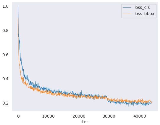
You can plot loss/mAP curves given a training log file. Run pip install seaborn first to install the dependency.
 loss curve image
python tools/analysis_tools/analyze_logs.py plot_curve [--keys ${KEYS}] [--title ${TITLE}] [--legend ${LEGEND}] [--backend ${BACKEND}] [--style ${STYLE}] [--out ${OUT_FILE}] [--mode ${MODE}] [--interval ${INTERVAL}]
Notice: If the metric you want to plot is calculated in the eval stage, you need to add the flag --mode eval. If you perform evaluation with an interval of ${INTERVAL}, you need to add the args --interval ${INTERVAL}.
Examples:
Plot the classification loss of some run.
python tools/analysis_tools/analyze_logs.py plot_curve log.json --keys loss_cls --legend loss_cls
Plot the classification and regression loss of some run, and save the figure to a pdf.
python tools/analysis_tools/analyze_logs.py plot_curve log.json --keys loss_cls loss_bbox --out losses.pdf
Compare the bbox mAP of two runs in the same figure.
# evaluate PartA2 and second on KITTI according to Car_3D_moderate_strict
python tools/analysis_tools/analyze_logs.py plot_curve tools/logs/PartA2.log.json tools/logs/second.log.json --keys KITTI/Car_3D_moderate_strict --legend PartA2 second --mode eval --interval 1
# evaluate PointPillars for car and 3 classes on KITTI according to Car_3D_moderate_strict
python tools/analysis_tools/analyze_logs.py plot_curve tools/logs/pp-3class.log.json tools/logs/pp.log.json --keys KITTI/Car_3D_moderate_strict --legend pp-3class pp --mode eval --interval 2
You can also compute the average training speed.
python tools/analysis_tools/analyze_logs.py cal_train_time log.json [--include-outliers]
The output is expected to be like the following.
-----Analyze train time of work_dirs/some_exp/20190611_192040.log.json-----
slowest epoch 11, average time is 1.2024
fastest epoch 1, average time is 1.1909
time std over epochs is 0.0028
average iter time: 1.1959 s/iter
Visualization
Results
To see the prediction results of trained models, you can run the following command
python tools/test.py ${CONFIG_FILE} ${CKPT_PATH} --show --show-dir ${SHOW_DIR}
After running this command, plotted results including input data and the output of networks visualized on the input (e.g. ***_points.obj and ***_pred.obj in single-modality 3D detection task) will be saved in ${SHOW_DIR}.
To see the prediction results during evaluation, you can run the following command
python tools/test.py ${CONFIG_FILE} ${CKPT_PATH} --eval 'mAP' --eval-options 'show=True' 'out_dir=${SHOW_DIR}'
After running this command, you will obtain the input data, the output of networks and ground-truth labels visualized on the input (e.g. ***_points.obj, ***_pred.obj, ***_gt.obj, ***_img.png and ***_pred.png in multi-modality detection task) in ${SHOW_DIR}. When show is enabled, Open3D will be used to visualize the results online. If you are running test in remote server without GUI, the online visualization is not supported, you can set show=False to only save the output results in {SHOW_DIR}.
As for offline visualization, you will have two options.
To visualize the results with Open3D backend, you can run the following command
python tools/misc/visualize_results.py ${CONFIG_FILE} --result ${RESULTS_PATH} --show-dir ${SHOW_DIR}
Or you can use 3D visualization software such as the MeshLab to open these files under ${SHOW_DIR} to see the 3D detection output. Specifically, open ***_points.obj to see the input point cloud and open ***_pred.obj to see the predicted 3D bounding boxes. This allows the inference and results generation to be done in remote server and the users can open them on their host with GUI.
Notice: The visualization API is a little unstable since we plan to refactor these parts together with MMDetection in the future.
Dataset
We also provide scripts to visualize the dataset without inference. You can use tools/misc/browse_dataset.py to show loaded data and ground-truth online and save them on the disk. Currently we support single-modality 3D detection and 3D segmentation on all the datasets, multi-modality 3D detection on KITTI and SUN RGB-D, as well as monocular 3D detection on nuScenes. To browse the KITTI dataset, you can run the following command
python tools/misc/browse_dataset.py configs/_base_/datasets/kitti-3d-3class.py --task det --output-dir ${OUTPUT_DIR} --online
Notice: Once specifying --output-dir, the images of views specified by users will be saved when pressing _ESC_ in open3d window. If you don’t have a monitor, you can remove the --online flag to only save the visualization results and browse them offline.
To verify the data consistency and the effect of data augmentation, you can also add --aug flag to visualize the data after data augmentation using the command as below:
python tools/misc/browse_dataset.py configs/_base_/datasets/kitti-3d-3class.py --task det --aug --output-dir ${OUTPUT_DIR} --online
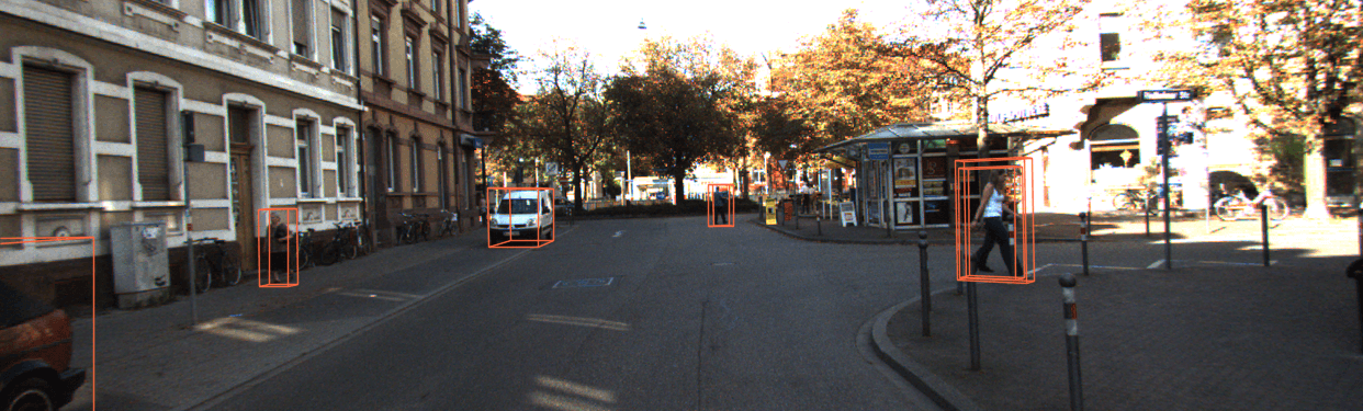
If you also want to show 2D images with 3D bounding boxes projected onto them, you need to find a config that supports multi-modality data loading, and then change the --task args to multi_modality-det. An example is showed below
python tools/misc/browse_dataset.py configs/mvxnet/dv_mvx-fpn_second_secfpn_adamw_2x8_80e_kitti-3d-3class.py --task multi_modality-det --output-dir ${OUTPUT_DIR} --online
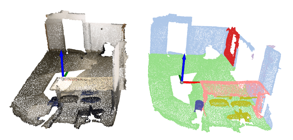
You can simply browse different datasets using different configs, e.g. visualizing the ScanNet dataset in 3D semantic segmentation task
python tools/misc/browse_dataset.py configs/_base_/datasets/scannet_seg-3d-20class.py --task seg --output-dir ${OUTPUT_DIR} --online
And browsing the nuScenes dataset in monocular 3D detection task
python tools/misc/browse_dataset.py configs/_base_/datasets/nus-mono3d.py --task mono-det --output-dir ${OUTPUT_DIR} --online
Model Serving
Note: This tool is still experimental now, only SECOND is supported to be served with TorchServe. We’ll support more models in the future.
In order to serve an MMDetection3D model with TorchServe, you can follow the steps:
1. Convert the model from MMDetection3D to TorchServe
python tools/deployment/mmdet3d2torchserve.py ${CONFIG_FILE} ${CHECKPOINT_FILE} \
--output-folder ${MODEL_STORE} \
--model-name ${MODEL_NAME}
Note: ${MODEL_STORE} needs to be an absolute path to a folder.
2. Build mmdet3d-serve docker image
docker build -t mmdet3d-serve:latest docker/serve/
3. Run mmdet3d-serve
Check the official docs for running TorchServe with docker.
In order to run it on the GPU, you need to install nvidia-docker. You can omit the --gpus argument in order to run on the CPU.
Example:
docker run --rm \
--cpus 8 \
--gpus device=0 \
-p8080:8080 -p8081:8081 -p8082:8082 \
--mount type=bind,source=$MODEL_STORE,target=/home/model-server/model-store \
mmdet3d-serve:latest
Read the docs about the Inference (8080), Management (8081) and Metrics (8082) APis
4. Test deployment
You can use test_torchserver.py to compare result of torchserver and pytorch.
python tools/deployment/test_torchserver.py ${IMAGE_FILE} ${CONFIG_FILE} ${CHECKPOINT_FILE} ${MODEL_NAME}
[--inference-addr ${INFERENCE_ADDR}] [--device ${DEVICE}] [--score-thr ${SCORE_THR}]
Example:
python tools/deployment/test_torchserver.py demo/data/kitti/kitti_000008.bin configs/second/hv_second_secfpn_6x8_80e_kitti-3d-car.py checkpoints/hv_second_secfpn_6x8_80e_kitti-3d-car_20200620_230238-393f000c.pth second
Model Complexity
You can use tools/analysis_tools/get_flops.py in MMDetection3D, a script adapted from flops-counter.pytorch, to compute the FLOPs and params of a given model.
python tools/analysis_tools/get_flops.py ${CONFIG_FILE} [--shape ${INPUT_SHAPE}]
You will get the results like this.
==============================
Input shape: (40000, 4)
Flops: 5.78 GFLOPs
Params: 953.83 k
==============================
Note: This tool is still experimental and we do not guarantee that the number is absolutely correct. You may well use the result for simple comparisons, but double check it before you adopt it in technical reports or papers.
FLOPs are related to the input shape while parameters are not. The default input shape is (1, 40000, 4).
Some operators are not counted into FLOPs like GN and custom operators. Refer to
mmcv.cnn.get_model_complexity_info()for details.We currently only support FLOPs calculation of single-stage models with single-modality input (point cloud or image). We will support two-stage and multi-modality models in the future.
Model Conversion
RegNet model to MMDetection
tools/model_converters/regnet2mmdet.py convert keys in pycls pretrained RegNet models to
MMDetection style.
python tools/model_converters/regnet2mmdet.py ${SRC} ${DST} [-h]
Detectron ResNet to Pytorch
tools/detectron2pytorch.py in MMDetection could convert keys in the original detectron pretrained
ResNet models to PyTorch style.
python tools/detectron2pytorch.py ${SRC} ${DST} ${DEPTH} [-h]
Prepare a model for publishing
tools/model_converters/publish_model.py helps users to prepare their model for publishing.
Before you upload a model to AWS, you may want to
convert model weights to CPU tensors
delete the optimizer states and
compute the hash of the checkpoint file and append the hash id to the filename.
python tools/model_converters/publish_model.py ${INPUT_FILENAME} ${OUTPUT_FILENAME}
E.g.,
python tools/model_converters/publish_model.py work_dirs/faster_rcnn/latest.pth faster_rcnn_r50_fpn_1x_20190801.pth
The final output filename will be faster_rcnn_r50_fpn_1x_20190801-{hash id}.pth.
Dataset Conversion
tools/data_converter/ contains tools for converting datasets to other formats. Most of them convert datasets to pickle based info files, like kitti, nuscenes and lyft. Waymo converter is used to reorganize waymo raw data like KITTI style. Users could refer to them for our approach to converting data format. It is also convenient to modify them to use as scripts like nuImages converter.
To convert the nuImages dataset into COCO format, please use the command below:
python -u tools/data_converter/nuimage_converter.py --data-root ${DATA_ROOT} --version ${VERSIONS} \
                                                    --out-dir ${OUT_DIR} --nproc ${NUM_WORKERS} --extra-tag ${TAG}
--data-root: the root of the dataset, defaults to./data/nuimages.--version: the version of the dataset, defaults tov1.0-mini. To get the full dataset, please use--version v1.0-train v1.0-val v1.0-mini--out-dir: the output directory of annotations and semantic masks, defaults to./data/nuimages/annotations/.--nproc: number of workers for data preparation, defaults to4. Larger number could reduce the preparation time as images are processed in parallel.--extra-tag: extra tag of the annotations, defaults tonuimages. This can be used to separate different annotations processed in different time for study.
More details could be referred to the doc for dataset preparation and README for nuImages dataset.